Simulation Study 1
Model 4 Results
R. Noah Padgett
2022-01-10
Last updated: 2022-01-16
Checks: 4 2
Knit directory: Padgett-Dissertation/
This reproducible R Markdown analysis was created with workflowr (version 1.6.2). The Checks tab describes the reproducibility checks that were applied when the results were created. The Past versions tab lists the development history.
Great job! The global environment was empty. Objects defined in the global environment can affect the analysis in your R Markdown file in unknown ways. For reproduciblity it’s best to always run the code in an empty environment.
The command set.seed(20210401) was run prior to running the code in the R Markdown file. Setting a seed ensures that any results that rely on randomness, e.g. subsampling or permutations, are reproducible.
Great job! Recording the operating system, R version, and package versions is critical for reproducibility.
- model4
- study1-model4-ppd
To ensure reproducibility of the results, delete the cache directory study1_model4_results_cache and re-run the analysis. To have workflowr automatically delete the cache directory prior to building the file, set delete_cache = TRUE when running wflow_build() or wflow_publish().
Great job! Using relative paths to the files within your workflowr project makes it easier to run your code on other machines.
Tracking code development and connecting the code version to the results is critical for reproducibility. To start using Git, open the Terminal and type git init in your project directory.
This project is not being versioned with Git. To obtain the full reproducibility benefits of using workflowr, please see ?wflow_start.
# Load packages & utility functions
source("code/load_packages.R")
source("code/load_utility_functions.R")
# environment options
options(scipen = 999, digits=3)
# generate data for study 1
source("code/study_1/study_1_generate_data.R")
Simulated Data
# data parameters
paravec <- c(
  N = 500
  , J = 5 # N_items
  , C = 3 # N_cat
  , etaCor = .23
  , etasd1 = 1
  , etasd2 = sqrt(0.1)
  , lambda=0.7
  , nu=1.5
  , sigma.ei=0.25
  , rho1=0.1
)
# simulated then saved below
sim_tau <- matrix(
  c(-0.822, -0.751, -0.616, -0.392, -0.865,
    0.780, 0.882, 0.827, 1.030, 0.877),
  ncol=2, nrow=5
)
# Use parameters to simulate data
sim.data <- simulate_data_misclass(paravec, tau=sim_tau)
Describing the Observed (simulated) Data
d1 <- sim.data$Ysampled %>%
  as.data.frame() %>%
  select(contains("y")) %>%
  mutate(id = 1:n()) %>%
  pivot_longer(
    cols = contains("y"),
    names_to = c("item"),
    values_to = "Response"
  ) %>%
  mutate(item = ifelse(nchar(item) > 2, substr(item, 2, 3), substr(item, 2, 2)))
d2 <- sim.data$logt %>%
  as.data.frame() %>%
  select(contains("logt")) %>%
  mutate(id = 1:n()) %>%
  pivot_longer(
    cols = contains("logt"),
    names_to = c("item"),
    values_to = "Time"
  ) %>%
  mutate(item = ifelse(nchar(item) > 5, substr(item, 5, 6), substr(item, 5, 5)))
dat <- left_join(d1, d2)
Joining, by = c("id", "item")dat_sum <- dat %>%
select(item, Response, Time) %>%
group_by(item) %>%
summarize(
p1 = table(Response)[1] / n(),
p2 = table(Response)[2] / n(),
p3 = table(Response)[3] / n(),
M1 = mean(Response, na.rm = T),
Mt = mean(Time, na.rm = T),
SDt = sd(Time, na.rm = T)
)
colnames(dat_sum) <-
c(
"Item",
"Prop. R == 1",
"Prop. R == 2",
"Prop. R == 3",
"Mean Response",
"Mean Response Time",
"SD Response Time"
)
dat_sum$Item <- paste0("item_", 1:N_items)
kable(dat_sum, format = "html", digits = 3) %>%
kable_styling(full_width = T)| Item | Prop. R == 1 | Prop. R == 2 | Prop. R == 3 | Mean Response | Mean Response Time | SD Response Time |
|---|---|---|---|---|---|---|
| item_1 | 0.308 | 0.404 | 0.288 | 1.98 | 1.39 | 0.597 |
| item_2 | 0.310 | 0.414 | 0.276 | 1.97 | 1.43 | 0.618 |
| item_3 | 0.338 | 0.386 | 0.276 | 1.94 | 1.43 | 0.613 |
| item_4 | 0.362 | 0.384 | 0.254 | 1.89 | 1.40 | 0.592 |
| item_5 | 0.292 | 0.422 | 0.286 | 1.99 | 1.36 | 0.582 |
# covariance among items
cov(sim.data$Ysampled)
y1 y2 y3 y4 y5
y1 0.5968 0.0634 0.0428 0.0640 0.0319
y2 0.0634 0.5860 0.0440 0.0364 0.0258
y3 0.0428 0.0440 0.6114 0.0394 0.0457
y4 0.0640 0.0364 0.0394 0.6055 0.0655
y5 0.0319 0.0258 0.0457 0.0655 0.5791# correlation matrix
psych::polychoric(sim.data$Ysampled)Call: psych::polychoric(x = sim.data$Ysampled)
Polychoric correlations
y1 y2 y3 y4 y5
y1 1.00
y2 0.14 1.00
y3 0.09 0.09 1.00
y4 0.13 0.08 0.08 1.00
y5 0.07 0.05 0.09 0.14 1.00
with tau of
1 2
y1 -0.50 0.56
y2 -0.50 0.59
y3 -0.42 0.59
y4 -0.35 0.66
y5 -0.55 0.57Model 4: Full IFA with Misclassification
Model details
cat(read_file(paste0(w.d, "/code/study_1/model_4.txt")))model {
### Model
for(p in 1:N){
for(i in 1:nit){
# data model
y[p,i] ~ dcat(omega[p,i, ])
# LRV
ystar[p,i] ~ dnorm(lambda[i]*eta[p], 1)
# Pr(nu = 3)
pi[p,i,3] = phi(ystar[p,i] - tau[i,2])
# Pr(nu = 2)
pi[p,i,2] = phi(ystar[p,i] - tau[i,1]) - phi(ystar[p,i] - tau[i,2])
# Pr(nu = 1)
pi[p,i,1] = 1 - phi(ystar[p,i] - tau[i,1])
# log-RT model
dev[p,i]<-lambda[i]*(eta[p] - (tau[i,1]+tau[i,2])/2)
mu.lrt[p,i] <- icept[i] - speed[p] - rho * abs(dev[p,i])
lrt[p,i] ~ dnorm(mu.lrt[p,i], prec[i])
# MISCLASSIFICATION MODEL
for(c in 1:ncat){
# generate informative prior for misclassificaiton
# parameters based on RT
for(ct in 1:ncat){
alpha[p,i,ct,c] <- ifelse(c == ct,
ilogit(lrt[p,i]),
(1/(ncat-1))*(1-ilogit(lrt[p,i]))
)
}
# sample misclassification parameters using the informative priors
gamma[p,i,c,1:ncat] ~ ddirch(alpha[p,i,c,1:ncat])
# observed category prob (Pr(y=c))
omega[p,i, c] = gamma[p,i,c,1]*pi[p,i,1] +
gamma[p,i,c,2]*pi[p,i,2] +
gamma[p,i,c,3]*pi[p,i,3]
}
}
}
### Priors
# person parameters
for(p in 1:N){
eta[p] ~ dnorm(0, 1) # latent ability
speed[p]~dnorm(sigma.ts*eta[p],prec.s) # latent speed
}
sigma.ts ~ dnorm(0, 0.1)
prec.s ~ dgamma(.1,.1)
for(i in 1:nit){
# lrt parameters
icept[i]~dnorm(0,.1)
prec[i]~dgamma(.1,.1)
# Thresholds
tau[i, 1] ~ dnorm(0.0,0.1)
tau[i, 2] ~ dnorm(0, 0.1)T(tau[i, 1],)
# loadings
lambda[i] ~ dnorm(0, .44)T(0,)
# LRV total variance
# total variance = residual variance + fact. Var.
theta[i] = 1 + pow(lambda[i],2)
# standardized loading
lambda.std[i] = lambda[i]/pow(theta[i],0.5)
}
rho~dnorm(0,.1)I(0,)
# compute omega
lambda_sum[1] = lambda[1]
for(i in 2:nit){
#lambda_sum (sum factor loadings)
lambda_sum[i] = lambda_sum[i-1]+lambda[i]
}
reli.omega = (pow(lambda_sum[nit],2))/(pow(lambda_sum[nit],2)+nit)
}Model results
# Save parameters
jags.params <- c("tau",
                 "lambda","lambda.std",
                 "theta",
                 "icept",
                 "prec",
                 "prec.s",
                 "sigma.ts",
                 "rho",
                 "reli.omega")
# initial-values
jags.inits <- function(){
    list(
      "tau"=matrix(c(-0.822, -0.751, -0.616, -0.392, -0.865,
                     0.780, 0.882, 0.827, 1.030, 0.877),
                   ncol=2, nrow=5),
      "lambda"=rep(0.7,5),
      "rho"=0.1,
      "icept"=rep(1.5, 5),
      "prec.s"=10,
      "prec"=rep(4, 5),
      "sigma.ts"=0.1,
      "eta"=sim.data$eta[,1,drop=T],
      "speed"=sim.data$eta[,2,drop=T],
      "ystar"=t(sim.data$ystar)
    )
  }
mydata <- list(
  y = sim.data$Ysampled,
  lrt = sim.data$logt,
  N = nrow(sim.data$Ysampled),
  nit = ncol(sim.data$Ysampled),
  ncat = 3
)

# Run model
model.fit <-  R2jags::jags(
  model = paste0(w.d, "/code/study_1/model_4.txt"),
  parameters.to.save = jags.params,
  inits = jags.inits,
  data = mydata,
  n.chains = 4,
  n.burnin = 5000,
  n.iter = 10000
)
module glm loadedCompiling model graph
Resolving undeclared variables
Allocating nodes
Graph information:
Observed stochastic nodes: 5000
Unobserved stochastic nodes: 11028
Total graph size: 124086
Initializing modelprint(model.fit, width=1000)Inference for Bugs model at "C:/Users/noahp/Documents/GitHub/Padgett-Dissertation/code/study_1/model_4.txt", fit using jags,
4 chains, each with 10000 iterations (first 5000 discarded), n.thin = 5
n.sims = 4000 iterations saved
mu.vect sd.vect 2.5% 25% 50% 75% 97.5% Rhat n.eff
icept[1] 1.564 0.067 1.436 1.519 1.563 1.609 1.703 1.02 140
icept[2] 1.595 0.081 1.455 1.536 1.588 1.648 1.768 1.08 36
icept[3] 1.651 0.097 1.469 1.581 1.650 1.721 1.843 1.06 45
icept[4] 1.587 0.069 1.461 1.538 1.586 1.632 1.724 1.04 60
icept[5] 1.535 0.078 1.396 1.478 1.530 1.586 1.695 1.08 37
lambda[1] 0.800 0.231 0.395 0.637 0.778 0.946 1.285 1.05 61
lambda[2] 0.689 0.220 0.273 0.540 0.689 0.833 1.133 1.07 56
lambda[3] 0.922 0.265 0.421 0.746 0.914 1.096 1.455 1.03 120
lambda[4] 0.760 0.218 0.406 0.608 0.734 0.884 1.270 1.03 99
lambda[5] 0.737 0.215 0.361 0.596 0.725 0.863 1.202 1.07 59
lambda.std[1] 0.607 0.110 0.367 0.538 0.614 0.687 0.789 1.04 74
lambda.std[2] 0.549 0.127 0.263 0.475 0.567 0.640 0.750 1.09 59
lambda.std[3] 0.658 0.113 0.388 0.598 0.675 0.739 0.824 1.05 160
lambda.std[4] 0.589 0.104 0.376 0.520 0.592 0.662 0.786 1.02 110
lambda.std[5] 0.577 0.110 0.339 0.512 0.587 0.653 0.769 1.10 59
prec[1] 4.010 0.305 3.451 3.804 3.996 4.211 4.640 1.00 1000
prec[2] 4.007 0.304 3.437 3.798 3.996 4.199 4.647 1.00 2600
prec[3] 4.166 0.367 3.515 3.915 4.134 4.391 4.947 1.01 260
prec[4] 4.126 0.310 3.556 3.916 4.116 4.329 4.759 1.00 590
prec[5] 4.611 0.368 3.932 4.359 4.592 4.854 5.353 1.00 1100
prec.s 10.676 1.717 8.082 9.488 10.402 11.600 14.668 1.06 51
reli.omega 0.747 0.051 0.633 0.714 0.753 0.784 0.829 1.02 180
rho 0.292 0.099 0.113 0.222 0.285 0.361 0.493 1.07 47
sigma.ts 0.089 0.032 0.027 0.068 0.089 0.111 0.152 1.00 2700
tau[1,1] -0.881 0.144 -1.175 -0.975 -0.877 -0.781 -0.616 1.02 120
tau[2,1] -0.877 0.139 -1.161 -0.969 -0.877 -0.782 -0.610 1.01 230
tau[3,1] -0.754 0.150 -1.071 -0.849 -0.744 -0.647 -0.484 1.04 69
tau[4,1] -0.497 0.124 -0.745 -0.580 -0.493 -0.411 -0.259 1.00 650
tau[5,1] -0.924 0.139 -1.209 -1.014 -0.919 -0.828 -0.662 1.00 1100
tau[1,2] 0.984 0.149 0.704 0.881 0.980 1.081 1.290 1.01 570
tau[2,2] 1.026 0.141 0.758 0.927 1.026 1.120 1.305 1.00 1200
tau[3,2] 1.078 0.146 0.804 0.978 1.070 1.173 1.386 1.01 420
tau[4,2] 1.240 0.165 0.943 1.129 1.233 1.341 1.590 1.05 63
tau[5,2] 1.026 0.145 0.749 0.928 1.023 1.122 1.322 1.02 120
theta[1] 1.693 0.396 1.156 1.406 1.605 1.896 2.650 1.07 49
theta[2] 1.523 0.314 1.074 1.292 1.475 1.694 2.283 1.05 61
theta[3] 1.921 0.514 1.177 1.556 1.835 2.201 3.116 1.03 86
theta[4] 1.625 0.376 1.165 1.370 1.539 1.781 2.612 1.04 88
theta[5] 1.590 0.355 1.130 1.355 1.526 1.745 2.446 1.04 73
deviance 7763.790 83.063 7599.841 7706.525 7765.563 7820.484 7922.176 1.00 970
For each parameter, n.eff is a crude measure of effective sample size,
and Rhat is the potential scale reduction factor (at convergence, Rhat=1).
DIC info (using the rule, pD = var(deviance)/2)
pD = 3441.7 and DIC = 11205.5
DIC is an estimate of expected predictive error (lower deviance is better).Posterior Distribution Summary
jags.mcmc <- as.mcmc(model.fit)
a <- colnames(as.data.frame(jags.mcmc[[1]]))
fit.mcmc <- data.frame(as.matrix(jags.mcmc, chains = T, iters = T))
colnames(fit.mcmc) <- c("chain", "iter", a)
fit.mcmc.ggs <- ggmcmc::ggs(jags.mcmc) # for GRB plot

# save posterior draws for later
write.csv(x=fit.mcmc, file=paste0(getwd(),"/data/study_1/posterior_draws_m4.csv"))
Categroy Thresholds (\(\tau\))
# tau
bayesplot::mcmc_areas(fit.mcmc, regex_pars = "tau", prob = 0.8); ggsave("fig/study1_model4_tau_dens.pdf")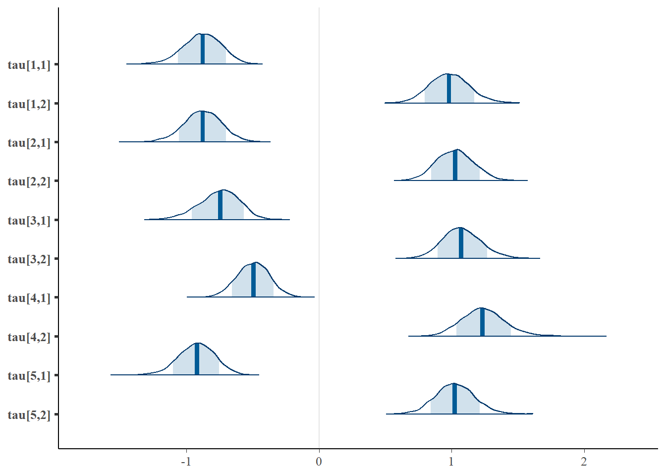
Saving 7 x 5 in imagebayesplot::mcmc_acf(fit.mcmc, regex_pars = "tau"); ggsave("fig/study1_model4_tau_acf.pdf")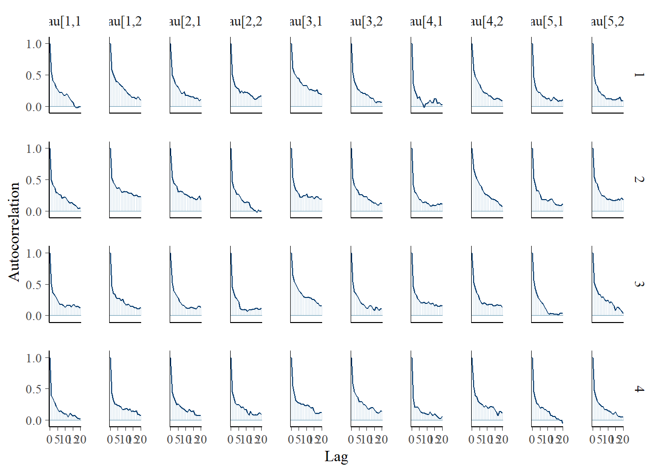
Saving 7 x 5 in imagebayesplot::mcmc_trace(fit.mcmc, regex_pars = "tau"); ggsave("fig/study1_model4_tau_trace.pdf")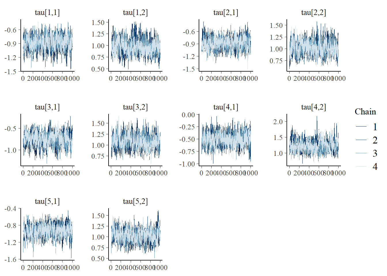
Saving 7 x 5 in imageggmcmc::ggs_grb(fit.mcmc.ggs, family = "tau"); ggsave("fig/study1_model4_tau_grb.pdf")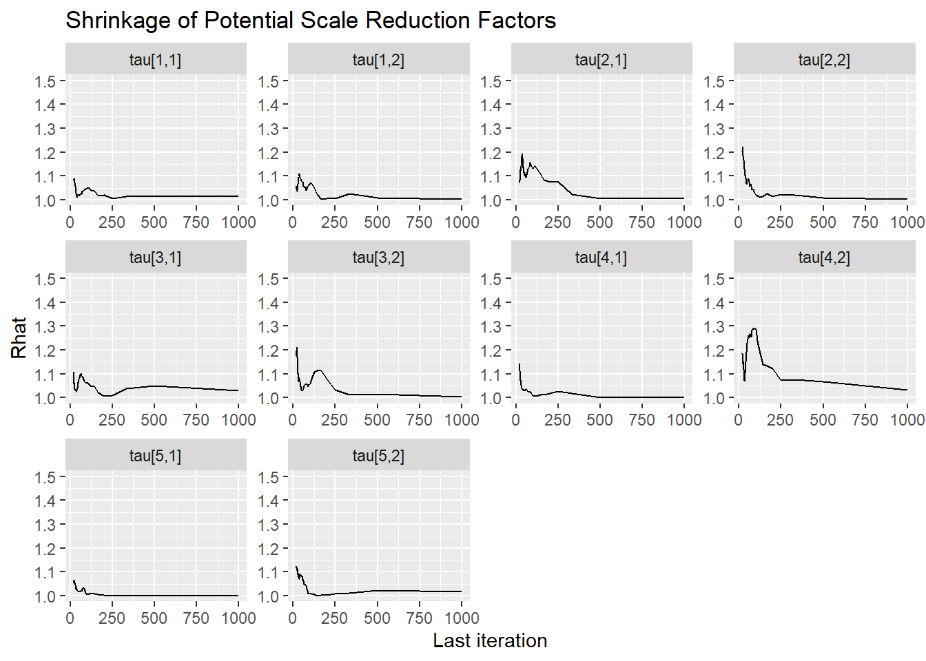
Saving 7 x 5 in imageFactor Loadings (\(\lambda\))
bayesplot::mcmc_areas(fit.mcmc, regex_pars = "lambda", prob = 0.8)
bayesplot::mcmc_acf(fit.mcmc, regex_pars = "lambda")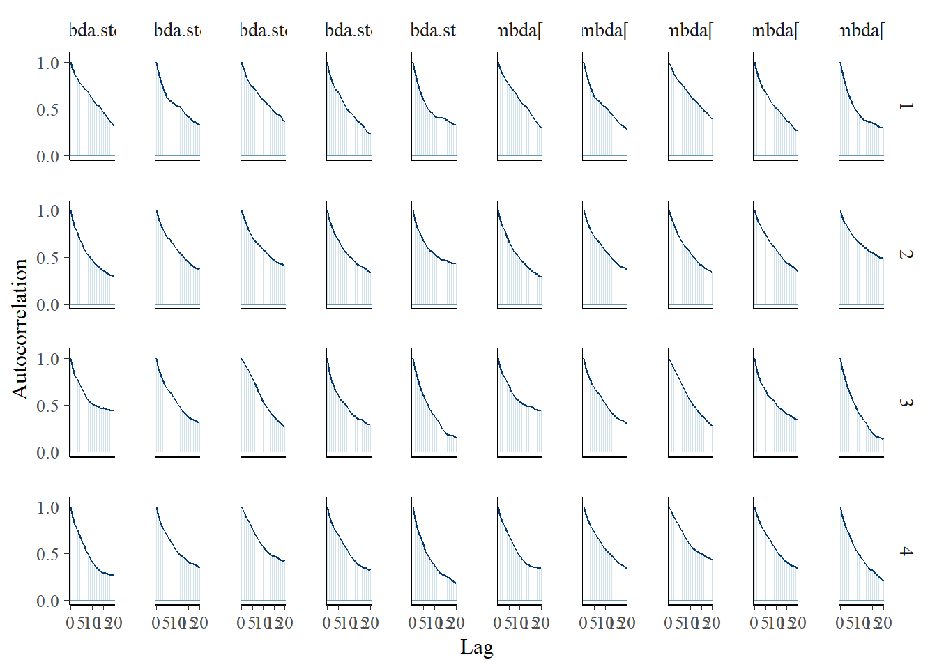
bayesplot::mcmc_trace(fit.mcmc, regex_pars = "lambda")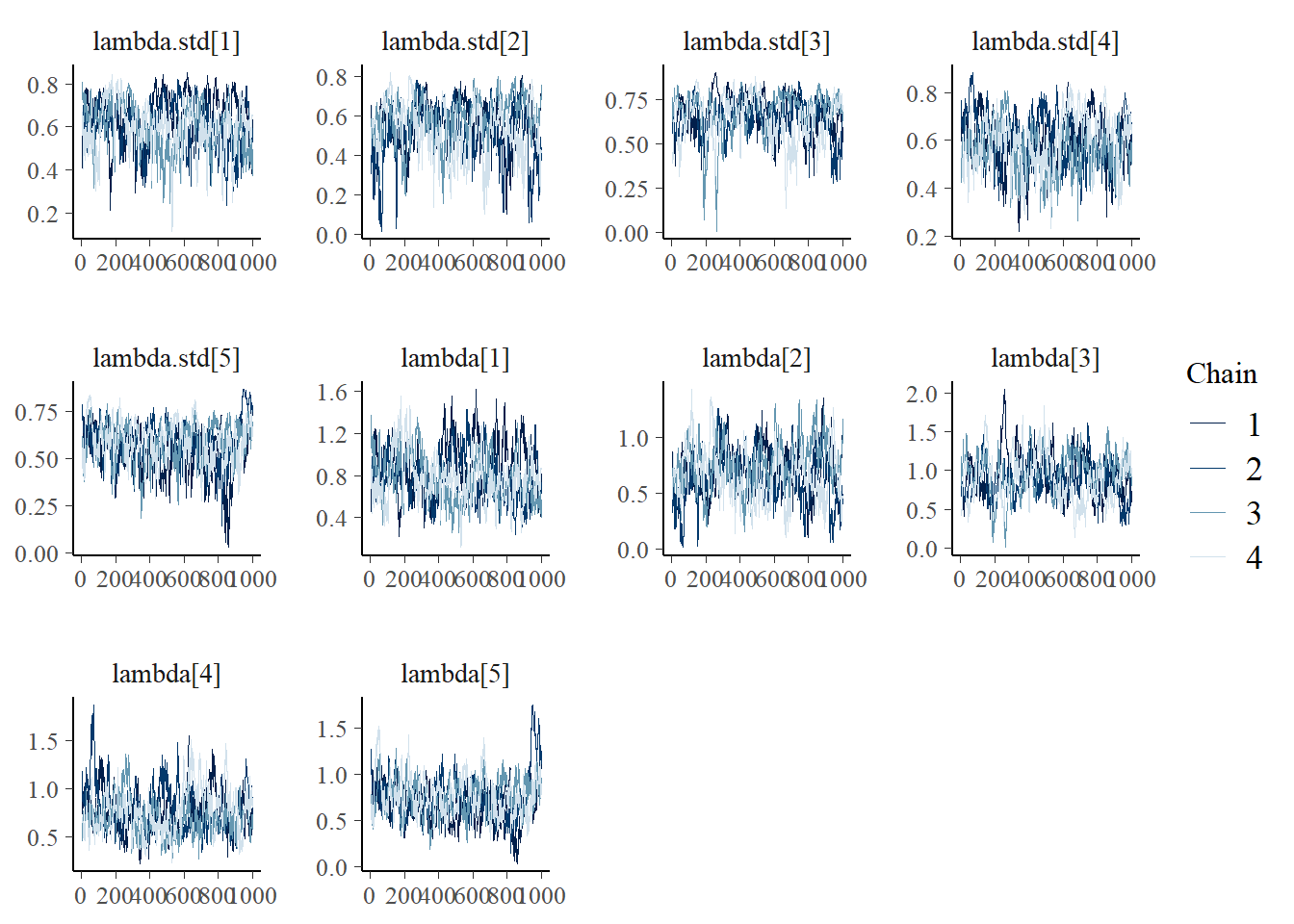
ggmcmc::ggs_grb(fit.mcmc.ggs, family = "lambda")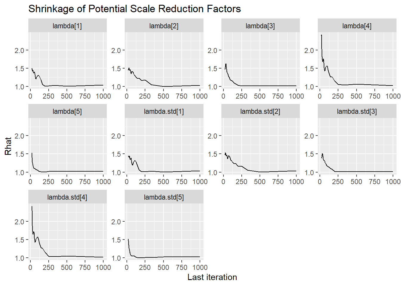
bayesplot::mcmc_areas(fit.mcmc, regex_pars = "lambda.std", prob = 0.8); ggsave("fig/study1_model4_lambda_dens.pdf")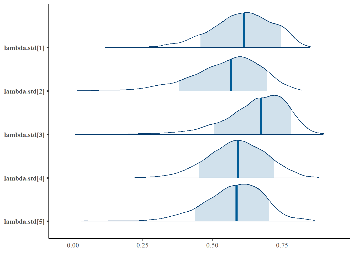
Saving 7 x 5 in imagebayesplot::mcmc_acf(fit.mcmc, regex_pars = "lambda.std"); ggsave("fig/study1_model4_lambda_acf.pdf")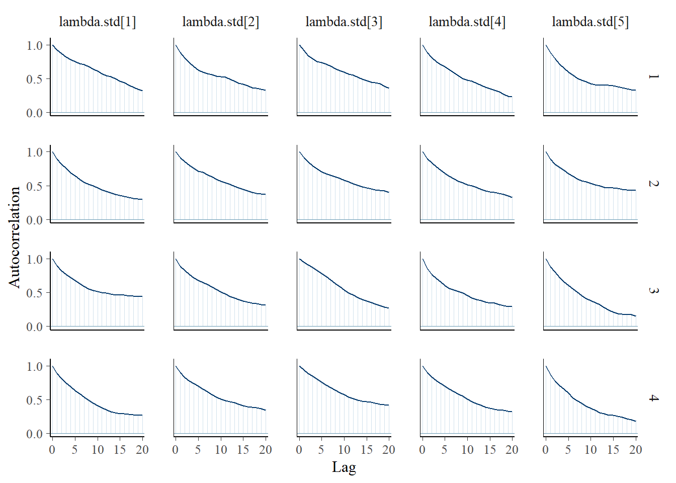
Saving 7 x 5 in imagebayesplot::mcmc_trace(fit.mcmc, regex_pars = "lambda.std"); ggsave("fig/study1_model4_lambda_trace.pdf")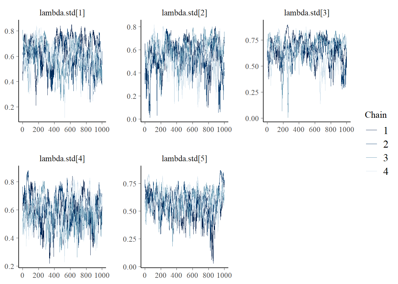
Saving 7 x 5 in imageggmcmc::ggs_grb(fit.mcmc.ggs, family = "lambda.std"); ggsave("fig/study1_model4_lambda_grb.pdf")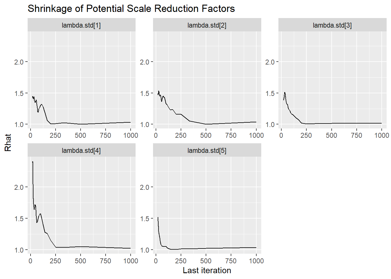
Saving 7 x 5 in imageLatent Response Total Variance (\(\theta\))
bayesplot::mcmc_areas(fit.mcmc, regex_pars = "theta", prob = 0.8); ggsave("fig/study1_model4_theta_dens.pdf")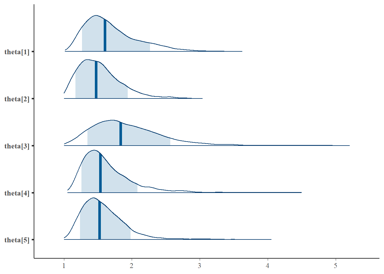
Saving 7 x 5 in imagebayesplot::mcmc_acf(fit.mcmc, regex_pars = "theta"); ggsave("fig/study1_model4_theta_acf.pdf")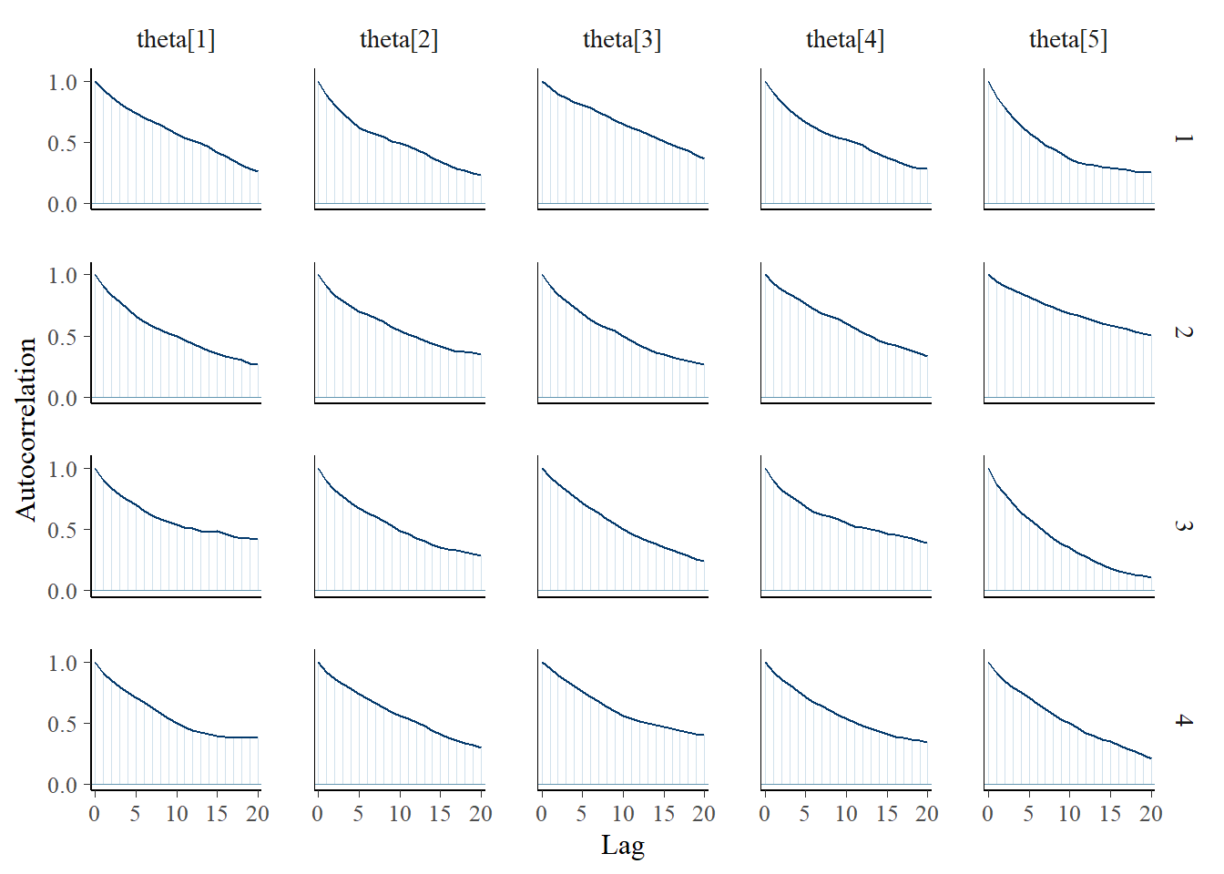
Saving 7 x 5 in imagebayesplot::mcmc_trace(fit.mcmc, regex_pars = "theta"); ggsave("fig/study1_model4_theta_trace.pdf")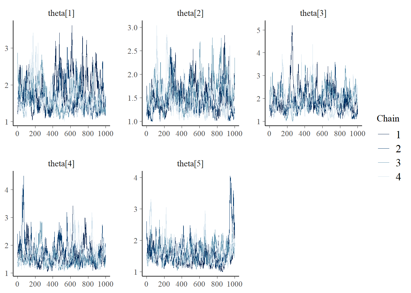
Saving 7 x 5 in imageggmcmc::ggs_grb(fit.mcmc.ggs, family = "theta"); ggsave("fig/study1_model4_theta_grb.pdf")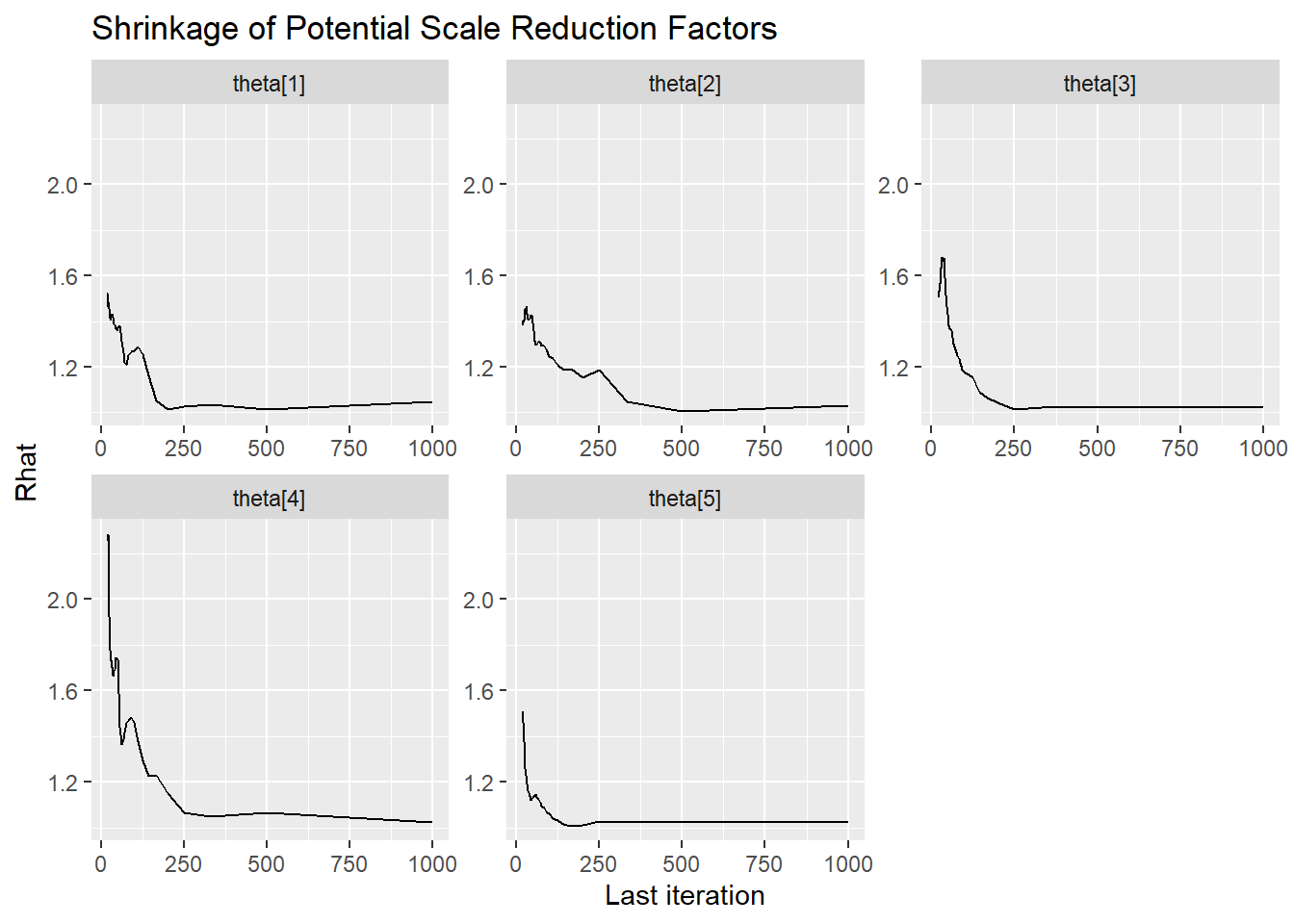
Saving 7 x 5 in imageResponse Time Intercept (\(\beta_{lrt}\))
bayesplot::mcmc_areas(fit.mcmc, regex_pars = "icept", prob = 0.8); ggsave("fig/study1_model4_icept_dens.pdf")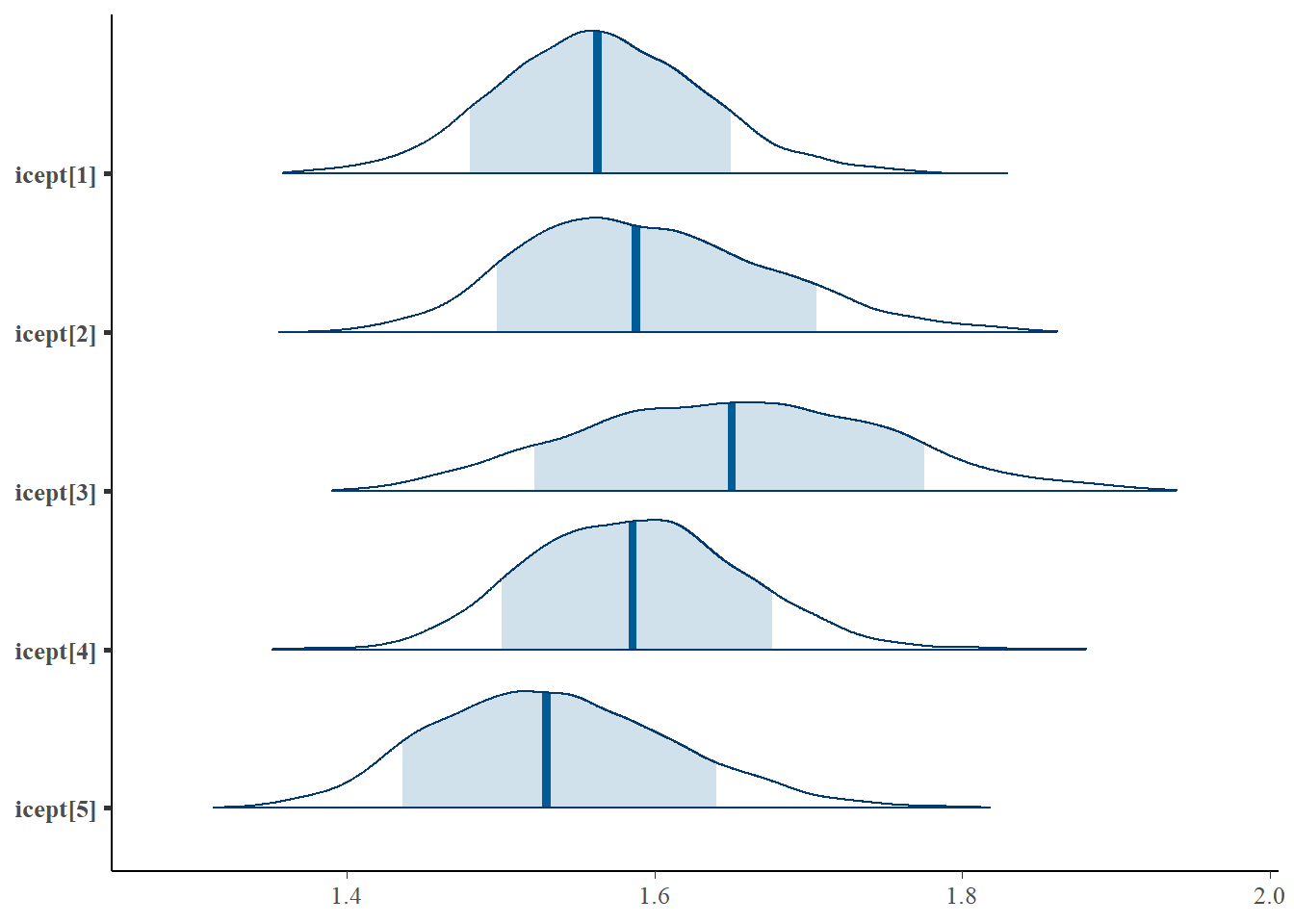
Saving 7 x 5 in imagebayesplot::mcmc_acf(fit.mcmc, regex_pars = "icept"); ggsave("fig/study1_model4_icept_acf.pdf")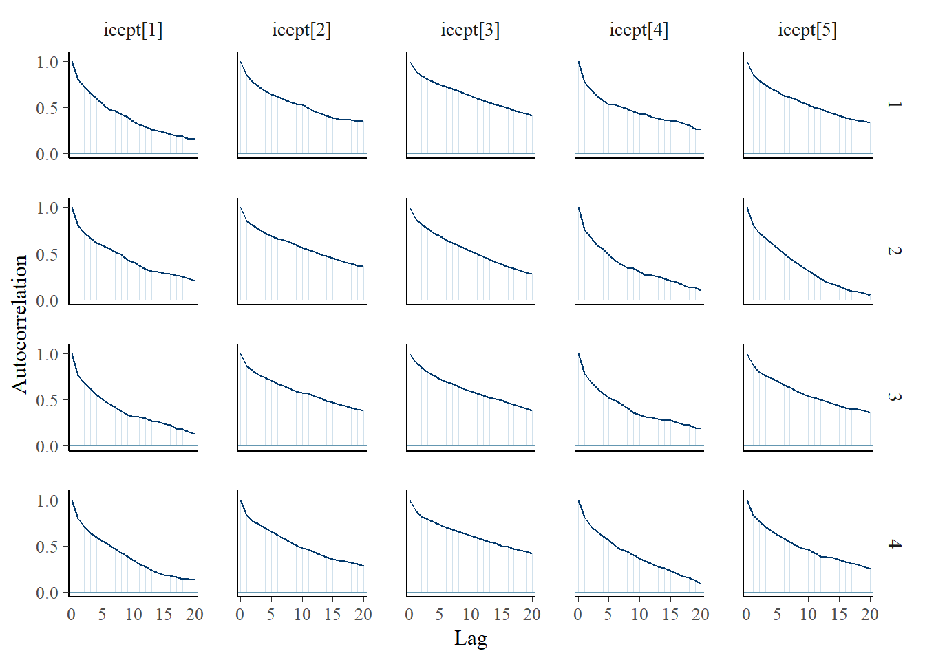
Saving 7 x 5 in imagebayesplot::mcmc_trace(fit.mcmc, regex_pars = "icept"); ggsave("fig/study1_model4_icept_trace.pdf")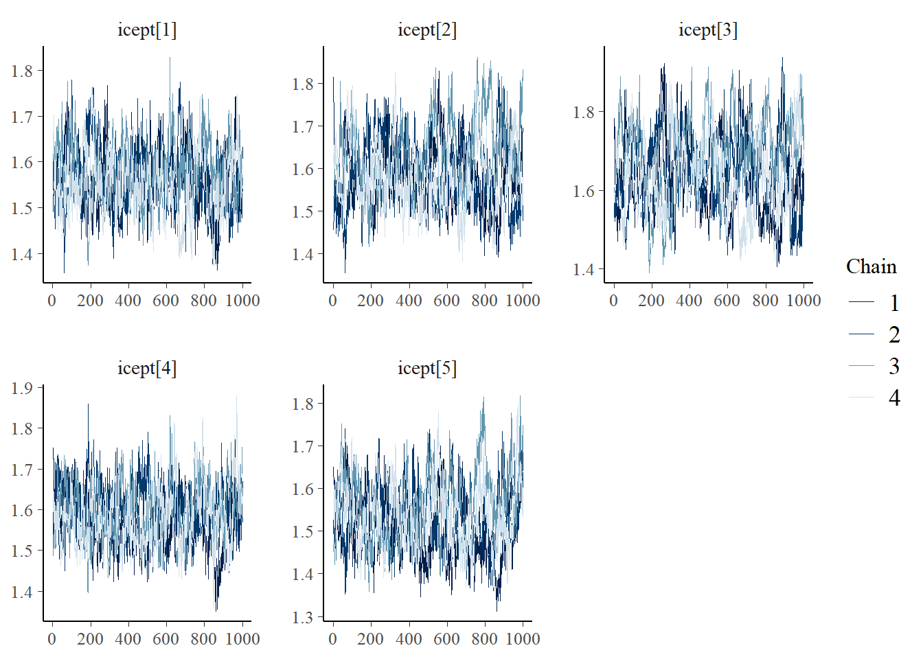
Saving 7 x 5 in imageggmcmc::ggs_grb(fit.mcmc.ggs, family = "icept"); ggsave("fig/study1_model4_icept_grb.pdf")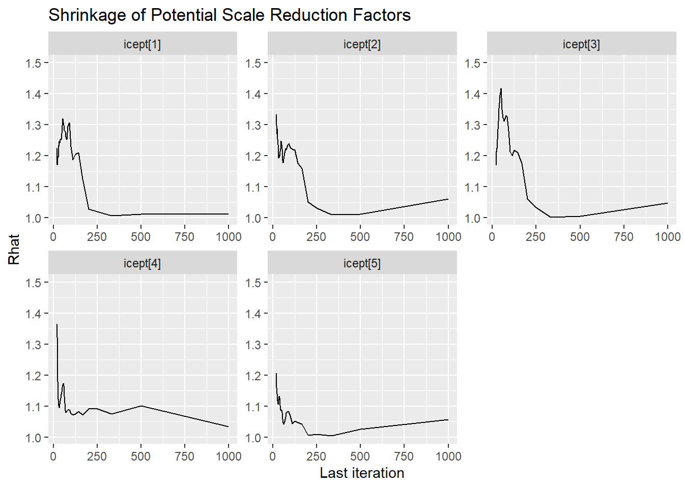
Saving 7 x 5 in imageResponse Time Precision (\(\sigma_{lrt}\))
bayesplot::mcmc_areas(fit.mcmc, regex_pars = "prec", prob = 0.8); ggsave("fig/study1_model4_prec_dens.pdf")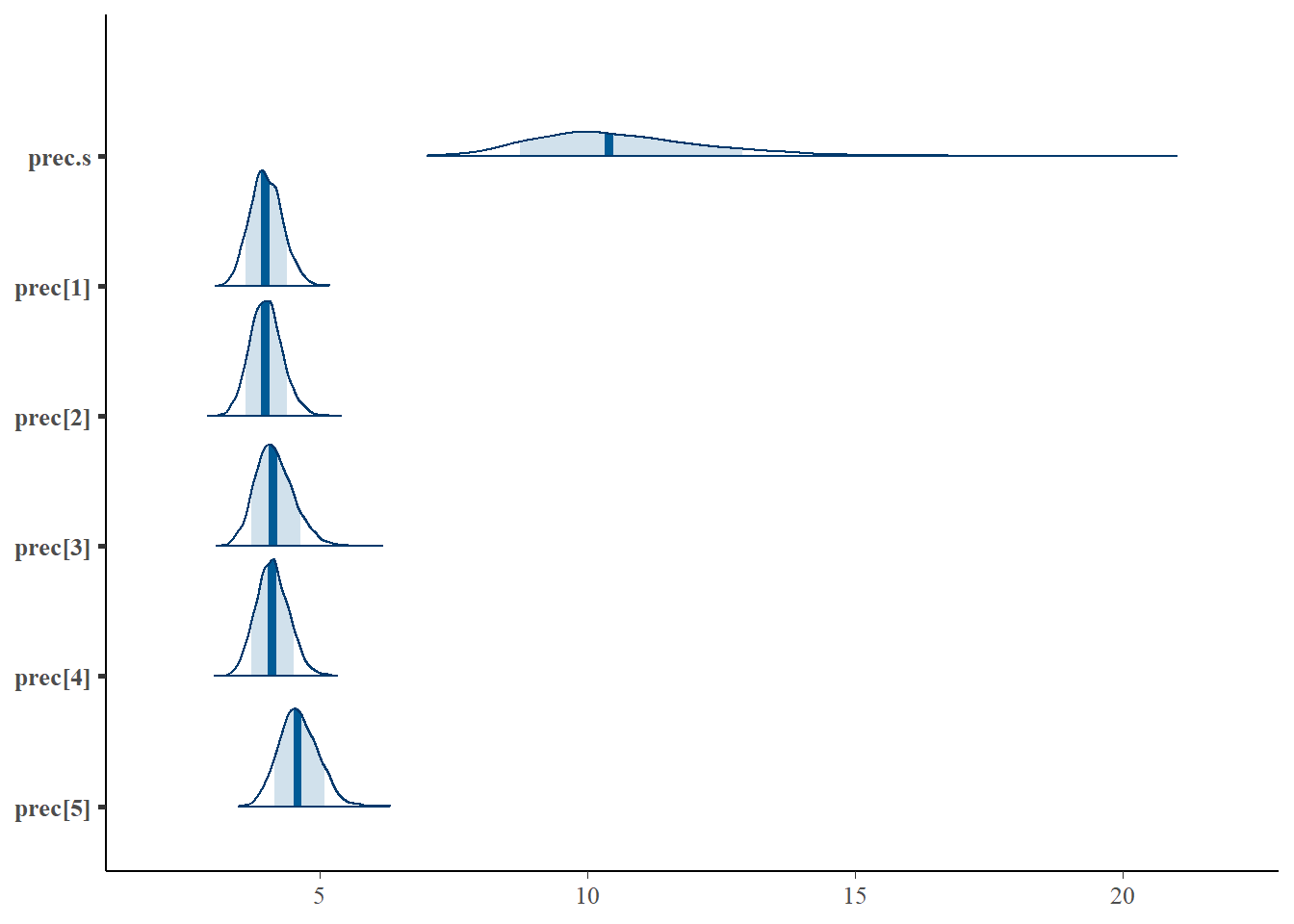
Saving 7 x 5 in imagebayesplot::mcmc_acf(fit.mcmc, regex_pars = "prec"); ggsave("fig/study1_model4_prec_acf.pdf")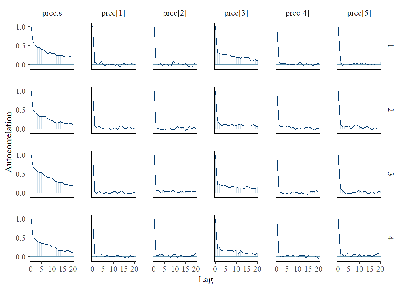
Saving 7 x 5 in imagebayesplot::mcmc_trace(fit.mcmc, regex_pars = "prec"); ggsave("fig/study1_model4_prec_trace.pdf")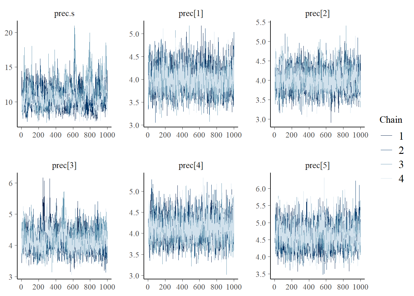
Saving 7 x 5 in imageggmcmc::ggs_grb(fit.mcmc.ggs, family = "prec"); ggsave("fig/study1_model4_prec_grb.pdf")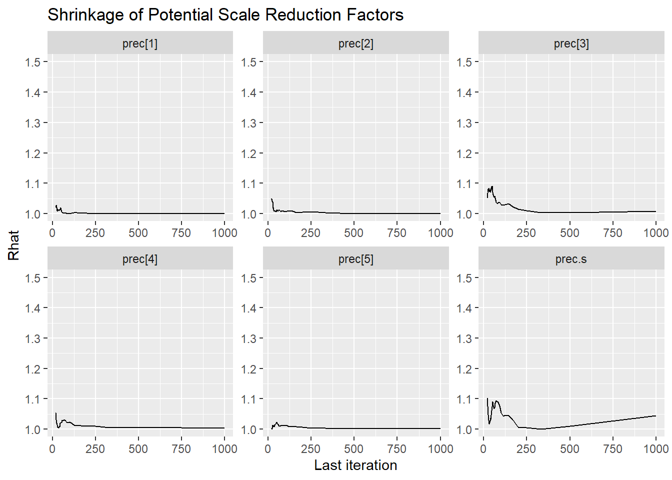
Saving 7 x 5 in imageSpeed Factor Variance (\(\sigma_s\))
bayesplot::mcmc_areas(fit.mcmc, regex_pars = "prec.s", prob = 0.8); ggsave("fig/study1_model4_precs_dens.pdf")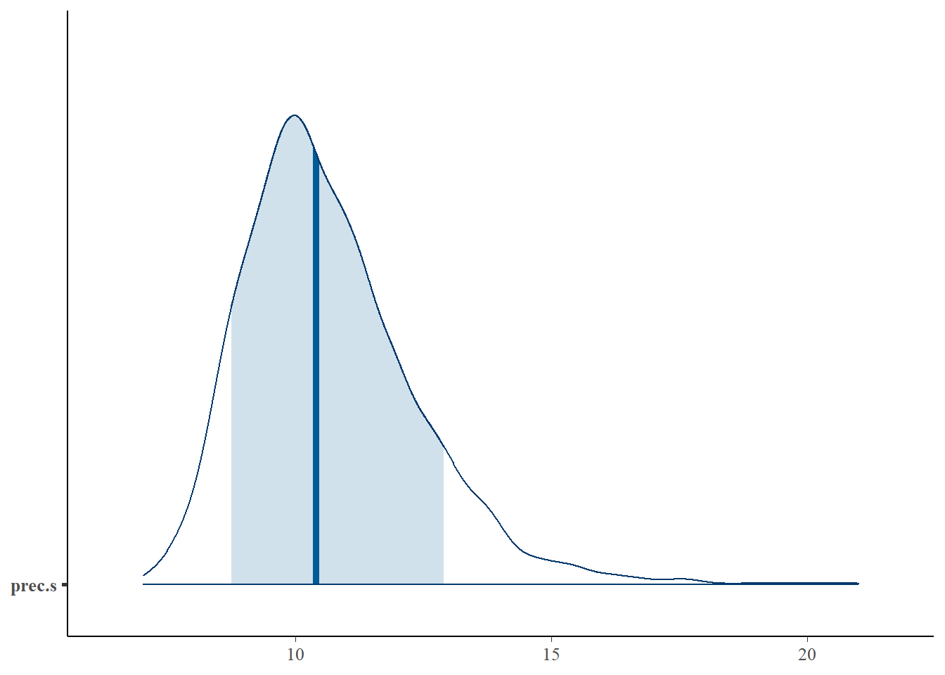
Saving 7 x 5 in imagebayesplot::mcmc_acf(fit.mcmc, regex_pars = "prec.s"); ggsave("fig/study1_model4_precs_acf.pdf")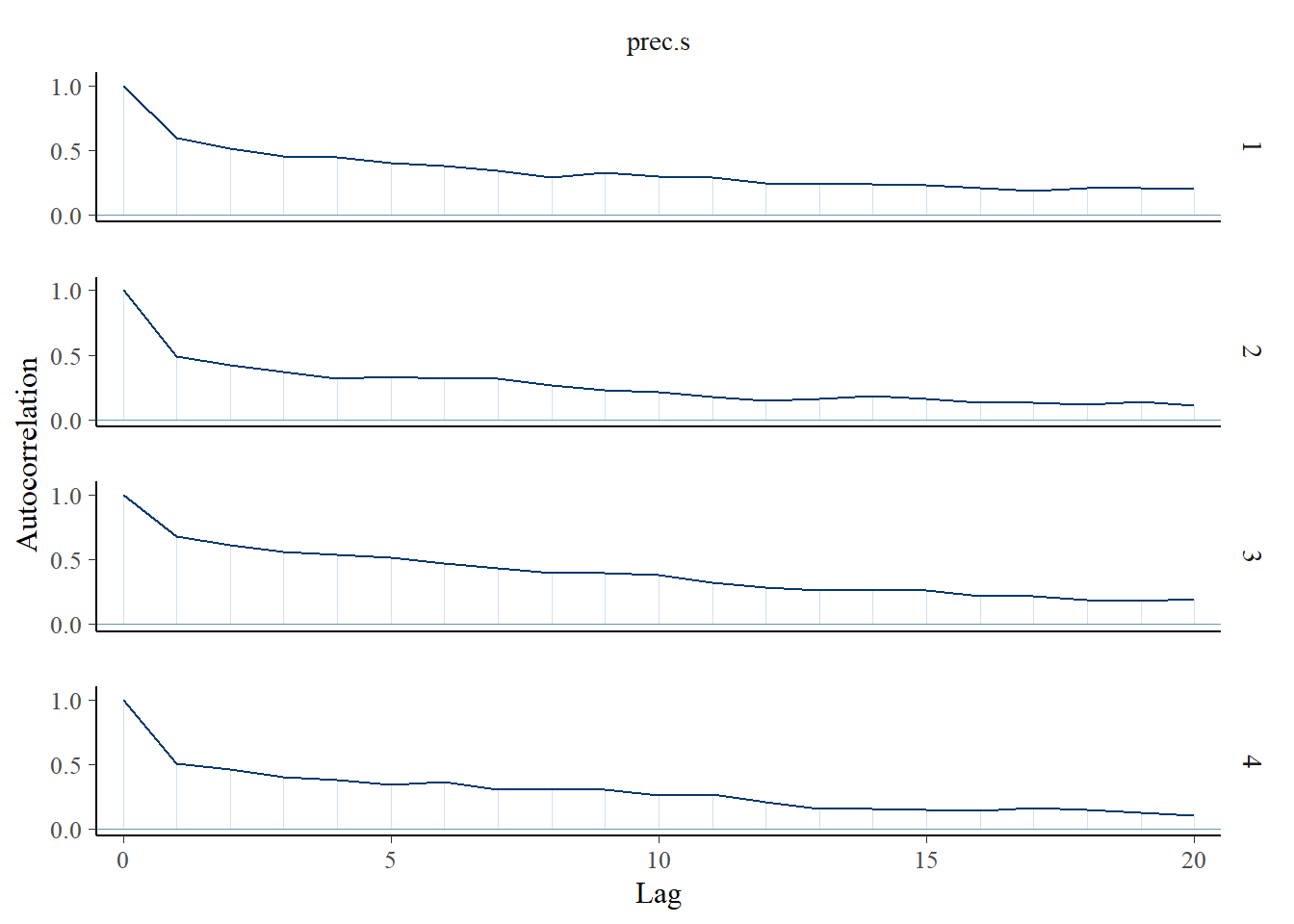
Saving 7 x 5 in imagebayesplot::mcmc_trace(fit.mcmc, regex_pars = "prec.s"); ggsave("fig/study1_model4_precs_trace.pdf")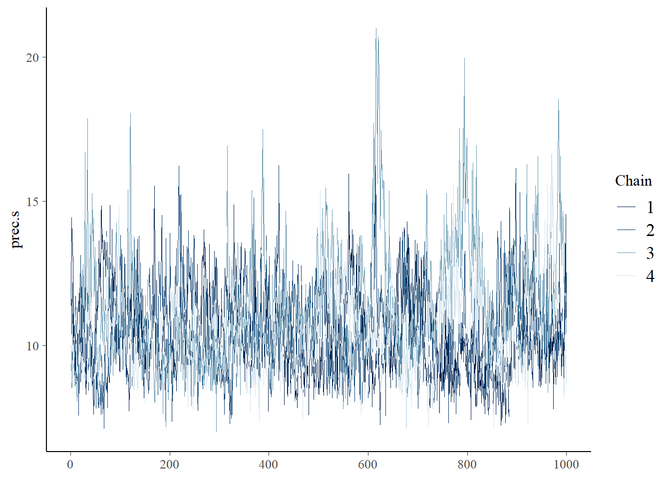
Saving 7 x 5 in imageggmcmc::ggs_grb(fit.mcmc.ggs, family = "prec.s"); ggsave("fig/study1_model4_precs_grb.pdf")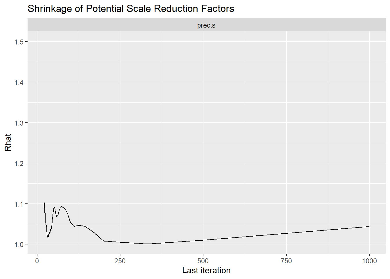
Saving 7 x 5 in imageFactor Covariance (\(\sigma_{ts}\))
bayesplot::mcmc_areas(fit.mcmc, regex_pars = "sigma.ts", prob = 0.8); ggsave("fig/study1_model4_sigmats_dens.pdf")
Saving 7 x 5 in imagebayesplot::mcmc_acf(fit.mcmc, regex_pars = "sigma.ts"); ggsave("fig/study1_model4_sigmats_acf.pdf")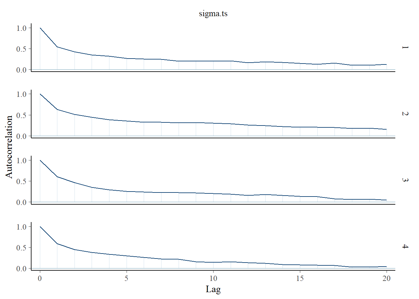
Saving 7 x 5 in imagebayesplot::mcmc_trace(fit.mcmc, regex_pars = "sigma.ts"); ggsave("fig/study1_model4_sigmats_trace.pdf")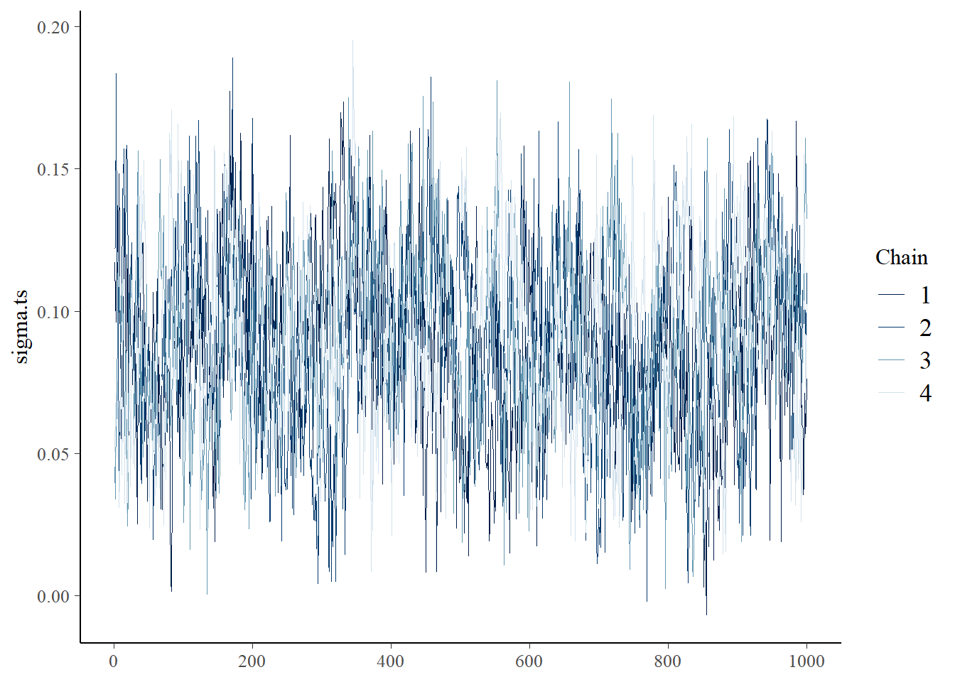
Saving 7 x 5 in imageggmcmc::ggs_grb(fit.mcmc.ggs, family = "sigma.ts"); ggsave("fig/study1_model4_sigmats_grb.pdf")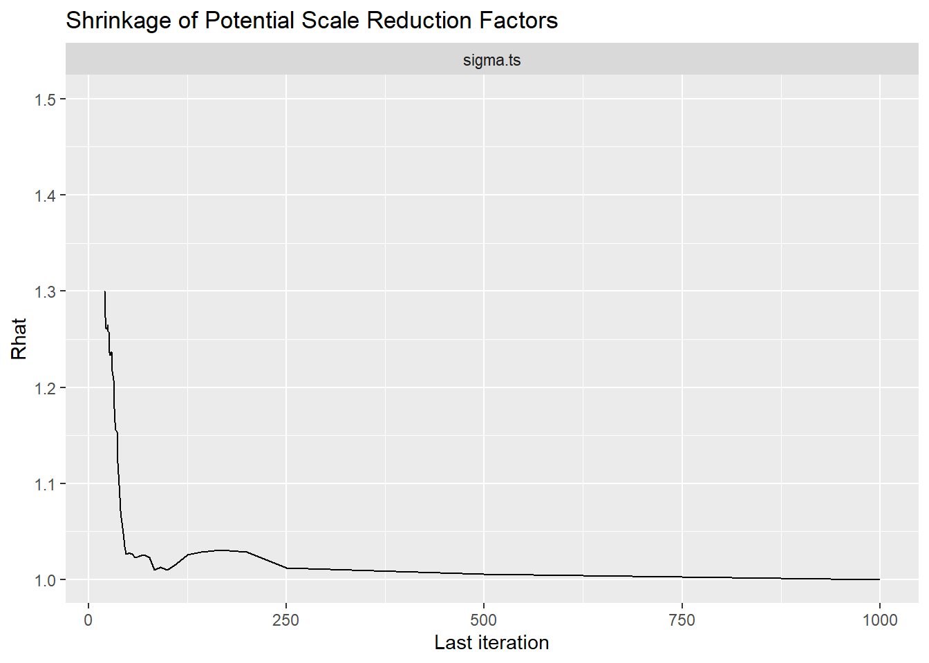
Saving 7 x 5 in imagePID (\(\rho\))
bayesplot::mcmc_areas(fit.mcmc, regex_pars = "rho", prob = 0.8); ggsave("fig/study1_model4_rho_dens.pdf")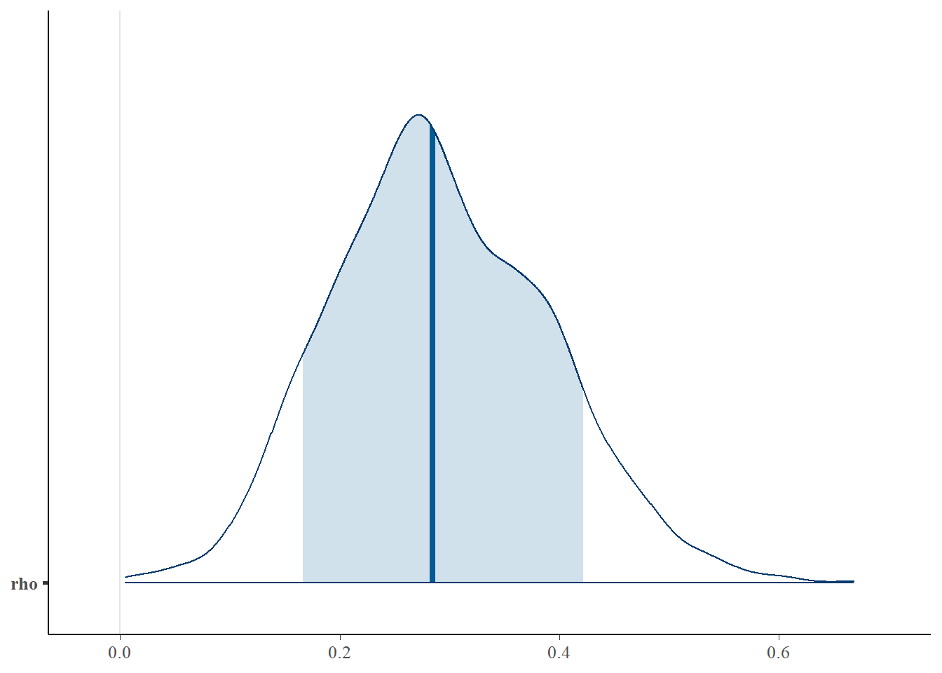
Saving 7 x 5 in imagebayesplot::mcmc_acf(fit.mcmc, regex_pars = "rho"); ggsave("fig/study1_model4_rho_acf.pdf")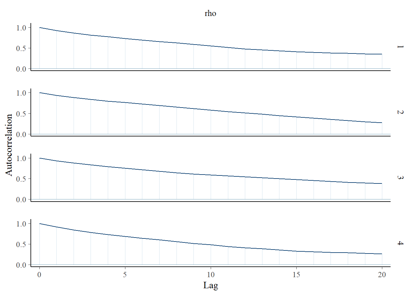
Saving 7 x 5 in imagebayesplot::mcmc_trace(fit.mcmc, regex_pars = "rho"); ggsave("fig/study1_model4_rho_trace.pdf")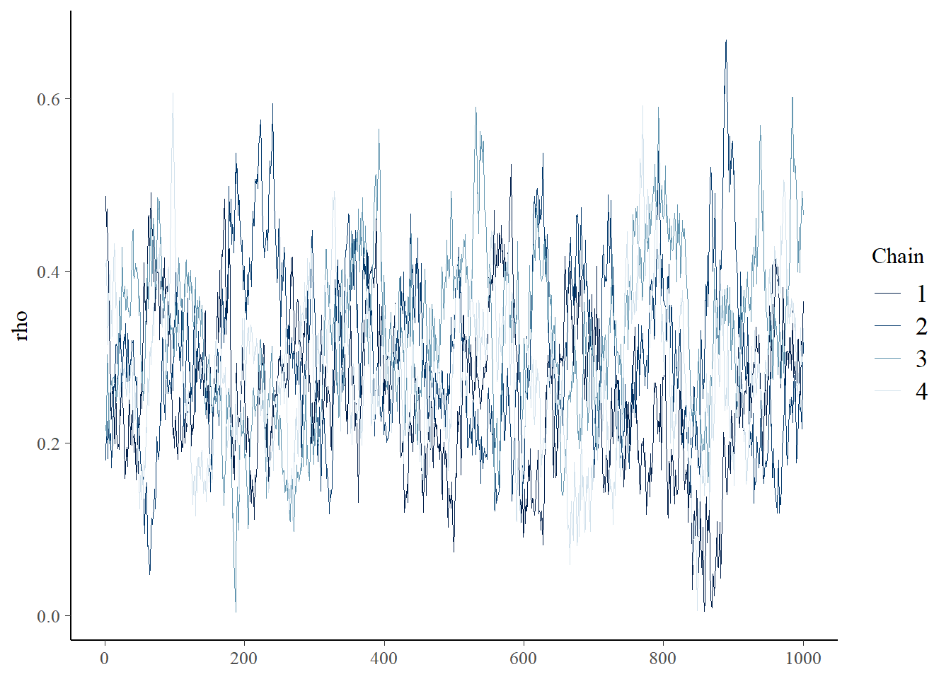
Saving 7 x 5 in imageggmcmc::ggs_grb(fit.mcmc.ggs, family = "rho"); ggsave("fig/study1_model4_rho_grb.pdf")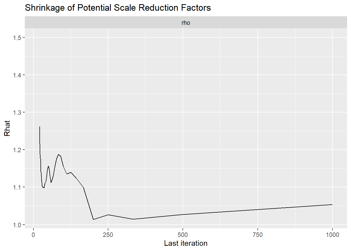
Saving 7 x 5 in imageFactor Reliability Omega (\(\omega\))
bayesplot::mcmc_areas(fit.mcmc, regex_pars = "reli.omega", prob = 0.8); ggsave("fig/study1_model4_omega_dens.pdf")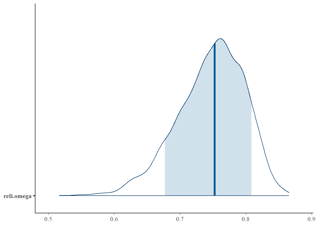
Saving 7 x 5 in imagebayesplot::mcmc_acf(fit.mcmc, regex_pars = "reli.omega"); ggsave("fig/study1_model4_omega_acf.pdf")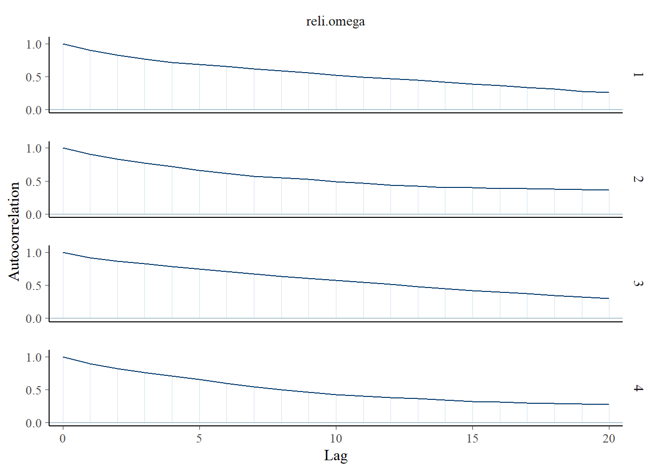
Saving 7 x 5 in imagebayesplot::mcmc_trace(fit.mcmc, regex_pars = "reli.omega"); ggsave("fig/study1_model4_omega_trace.pdf")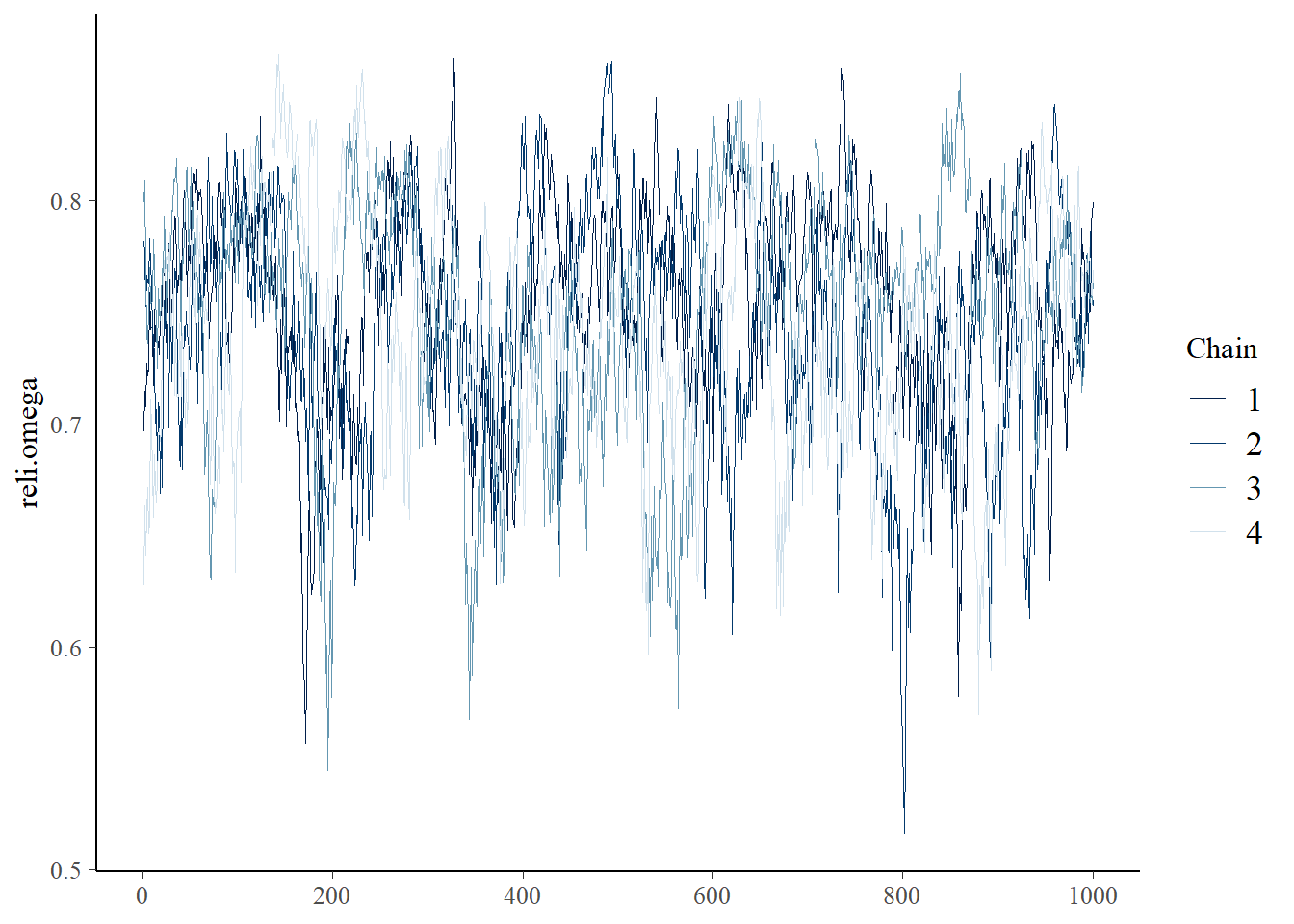
Saving 7 x 5 in imageggmcmc::ggs_grb(fit.mcmc.ggs, family = "reli.omega"); ggsave("fig/study1_model4_omega_grb.pdf")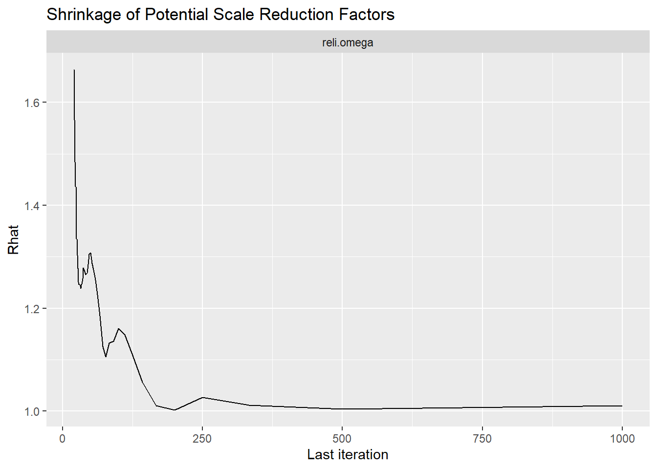
Saving 7 x 5 in image# extract omega posterior for results comparison
extracted_omega <- data.frame(model_4 = fit.mcmc$reli.omega)
write.csv(x=extracted_omega, file=paste0(getwd(),"/data/study_1/extracted_omega_m4.csv"))Posterior Predictive Distributions
# Posterior Predictive Check
Niter <- 200
model.fit$model$recompile()
Compiling model graph
Resolving undeclared variables
Allocating nodes
Graph information:
Observed stochastic nodes: 5000
Unobserved stochastic nodes: 11028
Total graph size: 124086
Initializing modelfit.extra <- rjags::jags.samples(model.fit$model, variable.names = "omega", n.iter = Niter)NOTE: Stopping adaptationN <- model.fit$model$data()[[1]]
nit <- 5
nchain=4
C <- 3
n <- i <- iter <- ppc.row.i <- 1
y.prob.ppc <- array(dim=c(Niter*nchain, nit, C))
for(chain in 1:nchain){
for(iter in 1:Niter){
# initialize simulated y for this iteration
y <- matrix(nrow=N, ncol=nit)
# loop over item
for(i in 1:nit){
# simulated data for item i for each person
for(n in 1:N){
y[n,i] <- sample(1:C, 1, prob = fit.extra$omega[n, i, 1:C, iter, chain])
}
# computer proportion of each response category
for(c in 1:C){
y.prob.ppc[ppc.row.i,i,c] <- sum(y[,i]==c)/N
}
}
# update row of output
ppc.row.i = ppc.row.i + 1
}
}
yppcmat <- matrix(c(y.prob.ppc), ncol=1)
z <- expand.grid(1:(Niter*nchain), 1:nit, 1:C)
yppcmat <- data.frame( iter = z[,1], nit=z[,2], C=z[,3], yppc = yppcmat)
ymat <- model.fit$model$data()[["y"]]
y.prob <- matrix(ncol=C, nrow=nit)
for(i in 1:nit){
for(c in 1:C){
y.prob[i,c] <- sum(ymat[,i]==c)/N
}
}
yobsmat <- matrix(c(y.prob), ncol=1)
z <- expand.grid(1:nit, 1:C)
yobsmat <- data.frame(nit=z[,1], C=z[,2], yobs = yobsmat)
plot.ppc <- full_join(yppcmat, yobsmat)Joining, by = c("nit", "C")p <- plot.ppc %>%
mutate(C = as.factor(C),
item = nit) %>%
ggplot()+
geom_boxplot(aes(x=C,y=y.prob.ppc), outlier.colour = NA)+
geom_point(aes(x=C,y=yobs), color="red")+
lims(y=c(0, 0.67))+
labs(y="Posterior Predictive Category Proportion", x="Item Category")+
facet_wrap(.~nit, nrow=1)+
theme_bw()+
theme(
panel.grid = element_blank(),
strip.background = element_rect(fill="white")
)
p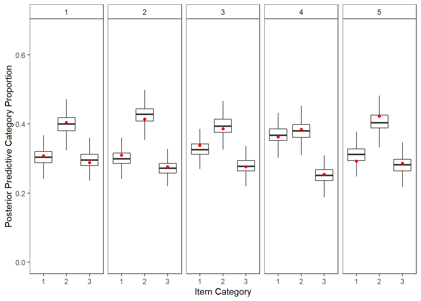
ggsave(filename = "fig/study1_model4_ppc_y.pdf",plot=p,width = 6, height=4,units="in")
ggsave(filename = "fig/study1_model4_ppc_y.png",plot=p,width = 6, height=4,units="in")
ggsave(filename = "fig/study1_model4_ppc_y.eps",plot=p,width = 6, height=4,units="in")
Manuscript Table and Figures
Table
# print to xtable
print(
  xtable(
    model.fit$BUGSoutput$summary,
    caption = c("study1 Model 4 posterior distribution summary")
    ,align = "lrrrrrrrrr"
  ),
  include.rownames=T,
  booktabs=T
)
% latex table generated in R 4.0.5 by xtable 1.8-4 package
% Sun Jan 16 13:45:08 2022
\begin{table}[ht]
\centering
\begin{tabular}{lrrrrrrrrr}
\toprule
& mean & sd & 2.5\% & 25\% & 50\% & 75\% & 97.5\% & Rhat & n.eff \\
\midrule
deviance & 7763.79 & 83.06 & 7599.84 & 7706.53 & 7765.56 & 7820.48 & 7922.18 & 1.00 & 970.00 \\
icept[1] & 1.56 & 0.07 & 1.44 & 1.52 & 1.56 & 1.61 & 1.70 & 1.02 & 140.00 \\
icept[2] & 1.60 & 0.08 & 1.45 & 1.54 & 1.59 & 1.65 & 1.77 & 1.08 & 36.00 \\
icept[3] & 1.65 & 0.10 & 1.47 & 1.58 & 1.65 & 1.72 & 1.84 & 1.06 & 45.00 \\
icept[4] & 1.59 & 0.07 & 1.46 & 1.54 & 1.59 & 1.63 & 1.72 & 1.05 & 60.00 \\
icept[5] & 1.53 & 0.08 & 1.40 & 1.48 & 1.53 & 1.59 & 1.70 & 1.08 & 37.00 \\
lambda[1] & 0.80 & 0.23 & 0.39 & 0.64 & 0.78 & 0.95 & 1.28 & 1.05 & 61.00 \\
lambda[2] & 0.69 & 0.22 & 0.27 & 0.54 & 0.69 & 0.83 & 1.13 & 1.07 & 56.00 \\
lambda[3] & 0.92 & 0.26 & 0.42 & 0.75 & 0.91 & 1.10 & 1.45 & 1.03 & 120.00 \\
lambda[4] & 0.76 & 0.22 & 0.41 & 0.61 & 0.73 & 0.88 & 1.27 & 1.03 & 99.00 \\
lambda[5] & 0.74 & 0.21 & 0.36 & 0.60 & 0.72 & 0.86 & 1.20 & 1.07 & 59.00 \\
lambda.std[1] & 0.61 & 0.11 & 0.37 & 0.54 & 0.61 & 0.69 & 0.79 & 1.04 & 74.00 \\
lambda.std[2] & 0.55 & 0.13 & 0.26 & 0.48 & 0.57 & 0.64 & 0.75 & 1.09 & 59.00 \\
lambda.std[3] & 0.66 & 0.11 & 0.39 & 0.60 & 0.67 & 0.74 & 0.82 & 1.05 & 160.00 \\
lambda.std[4] & 0.59 & 0.10 & 0.38 & 0.52 & 0.59 & 0.66 & 0.79 & 1.02 & 110.00 \\
lambda.std[5] & 0.58 & 0.11 & 0.34 & 0.51 & 0.59 & 0.65 & 0.77 & 1.10 & 59.00 \\
prec[1] & 4.01 & 0.30 & 3.45 & 3.80 & 4.00 & 4.21 & 4.64 & 1.00 & 1000.00 \\
prec[2] & 4.01 & 0.30 & 3.44 & 3.80 & 4.00 & 4.20 & 4.65 & 1.00 & 2600.00 \\
prec[3] & 4.17 & 0.37 & 3.51 & 3.91 & 4.13 & 4.39 & 4.95 & 1.01 & 260.00 \\
prec[4] & 4.13 & 0.31 & 3.56 & 3.92 & 4.12 & 4.33 & 4.76 & 1.00 & 590.00 \\
prec[5] & 4.61 & 0.37 & 3.93 & 4.36 & 4.59 & 4.85 & 5.35 & 1.00 & 1100.00 \\
prec.s & 10.68 & 1.72 & 8.08 & 9.49 & 10.40 & 11.60 & 14.67 & 1.06 & 51.00 \\
reli.omega & 0.75 & 0.05 & 0.63 & 0.71 & 0.75 & 0.78 & 0.83 & 1.02 & 180.00 \\
rho & 0.29 & 0.10 & 0.11 & 0.22 & 0.28 & 0.36 & 0.49 & 1.07 & 47.00 \\
sigma.ts & 0.09 & 0.03 & 0.03 & 0.07 & 0.09 & 0.11 & 0.15 & 1.00 & 2700.00 \\
tau[1,1] & -0.88 & 0.14 & -1.18 & -0.98 & -0.88 & -0.78 & -0.62 & 1.02 & 120.00 \\
tau[2,1] & -0.88 & 0.14 & -1.16 & -0.97 & -0.88 & -0.78 & -0.61 & 1.01 & 230.00 \\
tau[3,1] & -0.75 & 0.15 & -1.07 & -0.85 & -0.74 & -0.65 & -0.48 & 1.04 & 69.00 \\
tau[4,1] & -0.50 & 0.12 & -0.75 & -0.58 & -0.49 & -0.41 & -0.26 & 1.00 & 650.00 \\
tau[5,1] & -0.92 & 0.14 & -1.21 & -1.01 & -0.92 & -0.83 & -0.66 & 1.00 & 1100.00 \\
tau[1,2] & 0.98 & 0.15 & 0.70 & 0.88 & 0.98 & 1.08 & 1.29 & 1.01 & 570.00 \\
tau[2,2] & 1.03 & 0.14 & 0.76 & 0.93 & 1.03 & 1.12 & 1.31 & 1.00 & 1200.00 \\
tau[3,2] & 1.08 & 0.15 & 0.80 & 0.98 & 1.07 & 1.17 & 1.39 & 1.01 & 420.00 \\
tau[4,2] & 1.24 & 0.17 & 0.94 & 1.13 & 1.23 & 1.34 & 1.59 & 1.05 & 63.00 \\
tau[5,2] & 1.03 & 0.15 & 0.75 & 0.93 & 1.02 & 1.12 & 1.32 & 1.02 & 120.00 \\
theta[1] & 1.69 & 0.40 & 1.16 & 1.41 & 1.60 & 1.90 & 2.65 & 1.07 & 49.00 \\
theta[2] & 1.52 & 0.31 & 1.07 & 1.29 & 1.47 & 1.69 & 2.28 & 1.05 & 61.00 \\
theta[3] & 1.92 & 0.51 & 1.18 & 1.56 & 1.83 & 2.20 & 3.12 & 1.04 & 86.00 \\
theta[4] & 1.62 & 0.38 & 1.17 & 1.37 & 1.54 & 1.78 & 2.61 & 1.04 & 88.00 \\
theta[5] & 1.59 & 0.36 & 1.13 & 1.35 & 1.53 & 1.75 & 2.45 & 1.04 & 73.00 \\
\bottomrule
\end{tabular}
\caption{study1 Model 4 posterior distribution summary}
\end{table}Figure
plot.dat <- fit.mcmc %>%
  select(!c("iter", "deviance", "reli.omega"))%>%
  pivot_longer(
    cols= !c("chain"),
    names_to="variable",
    values_to="value"
  )

meas.var <- c(
        "lambda.std[1]", "theta[1]", "tau[1,1]", "tau[1,2]",
        "lambda.std[2]", "theta[2]", "tau[2,1]", "tau[2,2]",
        "lambda.std[3]", "theta[3]", "tau[3,1]", "tau[3,2]",
        "lambda.std[4]", "theta[4]", "tau[4,1]", "tau[4,2]",
        "lambda.std[5]", "theta[5]", "tau[5,1]", "tau[5,2]"
      )
plot.dat1 <- plot.dat %>%
  filter(variable %in% meas.var) %>%
  mutate(
    variable = factor(
      variable,
      levels = meas.var, ordered = T
    )
  )

spd.var <- c(
        "icept[1]", "icept[2]", "icept[3]", "icept[4]", "icept[5]",
        "prec[1]", "prec[2]", "prec[3]", "prec[4]", "prec[5]",
        "rho", "prec.s", "sigma.ts"
      )
plot.dat2 <- plot.dat %>%
  filter(variable %in% spd.var) %>%
  mutate(
    variable = factor(
      variable,
      levels = spd.var, ordered = T
    )
  )


p1 <- ggplot(plot.dat1, aes(x=value, group=variable))+
  geom_density(adjust=2)+
  facet_wrap(variable~., scales="free_y", ncol=4) +
  labs(x="Magnitude of Parameter",
       y="Posterior Density")+
  theme_bw()+
  theme(
    panel.grid = element_blank(),
    strip.background = element_rect(fill="white"),
    axis.text.y = element_blank(),
    axis.ticks.y = element_blank()
  )
p1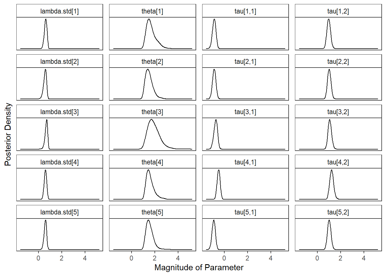
p2 <- ggplot(plot.dat2, aes(x=value, group=variable))+
  geom_density(adjust=2)+
  facet_wrap(variable~., scales="free", ncol=5) +
  labs(x="Magnitude of Parameter",
       y="Posterior Density")+
  theme_bw()+
  theme(
    panel.grid = element_blank(),
    strip.background = element_rect(fill="white"),
    axis.text.y = element_blank(),
    axis.ticks.y = element_blank() ,
    axis.text.x = element_text(size=8, angle=90, hjust=1, vjust=0.50)
  )
p2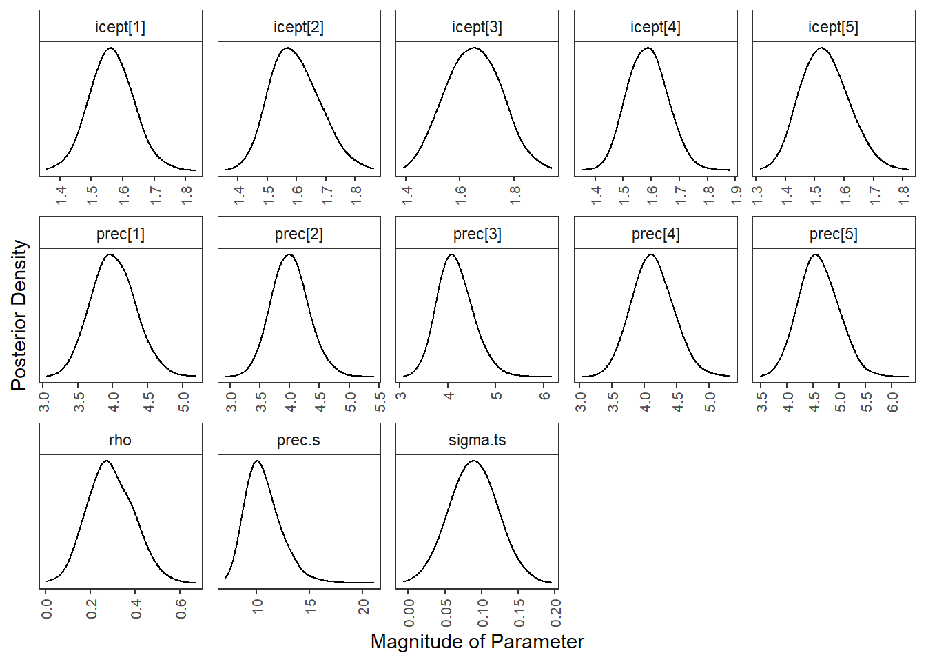
# all as one
plot.dat <- fit.mcmc %>%
  select(!c("iter", "deviance", "reli.omega", paste0("lambda[",1:5,"]")))%>%
  pivot_longer(
    cols= !c("chain"),
    names_to="variable",
    values_to="value"
  ) %>%
  mutate(
    variable = factor(
      variable,
      # 33
      # 10x3 + 3 === horizontal page
      levels = c(
        paste0("lambda.std[",1:5,"]"), paste0("theta[",1:5,"]"),
        paste0("tau[",1:5,",1]"), paste0("tau[",1:5,",2]"),
        paste0("icept[",1:5,"]"), paste0("prec[",1:5,"]"),
        "rho", "prec.s","sigma.ts"
      ), ordered = T
    )
  )
p <- ggplot(plot.dat, aes(x=value, group=variable))+
  geom_density(adjust=2)+
  facet_wrap(variable~., scales="free", ncol=5) +
  labs(x="Magnitude of Parameter",
       y="Posterior Density")+
  theme_bw()+
  theme(
    panel.grid = element_blank(),
    strip.background = element_rect(fill="white"),
    axis.text.y = element_blank(),
    axis.ticks.y = element_blank() ,
    axis.text.x = element_text(size=7)
  )
p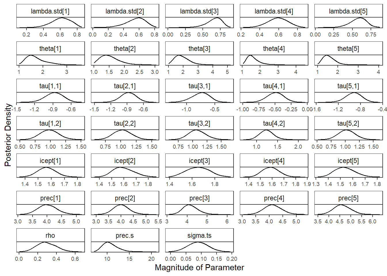
ggsave(filename = "fig/study1_model4_posterior_dist.pdf",plot=p,width = 10, height=7,units="in")
ggsave(filename = "fig/study1_model4_posterior_dist.png",plot=p,width = 10, height=7,units="in")
ggsave(filename = "fig/study1_model4_posterior_dist.eps",plot=p,width = 10, height=7,units="in")
sessionInfo()R version 4.0.5 (2021-03-31)
Platform: x86_64-w64-mingw32/x64 (64-bit)
Running under: Windows 10 x64 (build 22000)
Matrix products: default
locale:
[1] LC_COLLATE=English_United States.1252
[2] LC_CTYPE=English_United States.1252
[3] LC_MONETARY=English_United States.1252
[4] LC_NUMERIC=C
[5] LC_TIME=English_United States.1252
attached base packages:
[1] stats graphics grDevices utils datasets methods base
other attached packages:
[1] car_3.0-10 carData_3.0-4 mvtnorm_1.1-1
[4] LaplacesDemon_16.1.4 runjags_2.2.0-2 lme4_1.1-26
[7] Matrix_1.3-2 sirt_3.9-4 R2jags_0.6-1
[10] rjags_4-12 eRm_1.0-2 diffIRT_1.5
[13] statmod_1.4.35 xtable_1.8-4 kableExtra_1.3.4
[16] lavaan_0.6-7 polycor_0.7-10 bayesplot_1.8.0
[19] ggmcmc_1.5.1.1 coda_0.19-4 data.table_1.14.0
[22] patchwork_1.1.1 forcats_0.5.1 stringr_1.4.0
[25] dplyr_1.0.5 purrr_0.3.4 readr_1.4.0
[28] tidyr_1.1.3 tibble_3.1.0 ggplot2_3.3.5
[31] tidyverse_1.3.0 workflowr_1.6.2
loaded via a namespace (and not attached):
[1] minqa_1.2.4 TAM_3.5-19 colorspace_2.0-0 rio_0.5.26
[5] ellipsis_0.3.1 ggridges_0.5.3 rprojroot_2.0.2 fs_1.5.0
[9] rstudioapi_0.13 farver_2.1.0 fansi_0.4.2 lubridate_1.7.10
[13] xml2_1.3.2 splines_4.0.5 mnormt_2.0.2 knitr_1.31
[17] jsonlite_1.7.2 nloptr_1.2.2.2 broom_0.7.5 dbplyr_2.1.0
[21] compiler_4.0.5 httr_1.4.2 backports_1.2.1 assertthat_0.2.1
[25] cli_2.3.1 later_1.1.0.1 htmltools_0.5.1.1 tools_4.0.5
[29] gtable_0.3.0 glue_1.4.2 reshape2_1.4.4 Rcpp_1.0.7
[33] cellranger_1.1.0 jquerylib_0.1.3 vctrs_0.3.6 svglite_2.0.0
[37] nlme_3.1-152 psych_2.0.12 xfun_0.21 ps_1.6.0
[41] openxlsx_4.2.3 rvest_1.0.0 lifecycle_1.0.0 MASS_7.3-53.1
[45] scales_1.1.1 ragg_1.1.1 hms_1.0.0 promises_1.2.0.1
[49] parallel_4.0.5 RColorBrewer_1.1-2 curl_4.3 yaml_2.2.1
[53] sass_0.3.1 reshape_0.8.8 stringi_1.5.3 highr_0.8
[57] zip_2.1.1 boot_1.3-27 rlang_0.4.10 pkgconfig_2.0.3
[61] systemfonts_1.0.1 evaluate_0.14 lattice_0.20-41 labeling_0.4.2
[65] tidyselect_1.1.0 GGally_2.1.1 plyr_1.8.6 magrittr_2.0.1
[69] R6_2.5.0 generics_0.1.0 DBI_1.1.1 foreign_0.8-81
[73] pillar_1.5.1 haven_2.3.1 withr_2.4.1 abind_1.4-5
[77] modelr_0.1.8 crayon_1.4.1 utf8_1.1.4 tmvnsim_1.0-2
[81] rmarkdown_2.7 grid_4.0.5 readxl_1.3.1 CDM_7.5-15
[85] pbivnorm_0.6.0 git2r_0.28.0 reprex_1.0.0 digest_0.6.27
[89] webshot_0.5.2 httpuv_1.5.5 textshaping_0.3.1 stats4_4.0.5
[93] munsell_0.5.0 viridisLite_0.3.0 bslib_0.2.4 R2WinBUGS_2.1-21