Last updated: 2022-02-13

Checks: 5 1

Knit directory: Padgett-Dissertation/

This reproducible R Markdown analysis was created with workflowr (version 1.6.2). The Checks tab describes the reproducibility checks that were applied when the results were created. The Past versions tab lists the development history.

Environment: empty

Great job! The global environment was empty. Objects defined in the global environment can affect the analysis in your R Markdown file in unknown ways. For reproduciblity it’s best to always run the code in an empty environment.

Seed: set.seed(20210401)

The command set.seed(20210401) was run prior to running the code in the R Markdown file. Setting a seed ensures that any results that rely on randomness, e.g. subsampling or permutations, are reproducible.

Session information: recorded

Great job! Recording the operating system, R version, and package versions is critical for reproducibility.

Cache: none

Nice! There were no cached chunks for this analysis, so you can be confident that you successfully produced the results during this run.

File paths: relative

Great job! Using relative paths to the files within your workflowr project makes it easier to run your code on other machines.

Repository version: no version control

Tracking code development and connecting the code version to the results is critical for reproducibility. To start using Git, open the Terminal and type git init in your project directory.

This project is not being versioned with Git. To obtain the full reproducibility benefits of using workflowr, please see ?wflow_start.

# Load packages
source("code/load_packages.R")
source("code/load_utility_functions.R")
# environment options
options(scipen = 999, digits=3)

# results folder
res_folder <- paste0(w.d, "/data/study_2")

# read in data
source("code/load_extracted_data.R")

Convergence

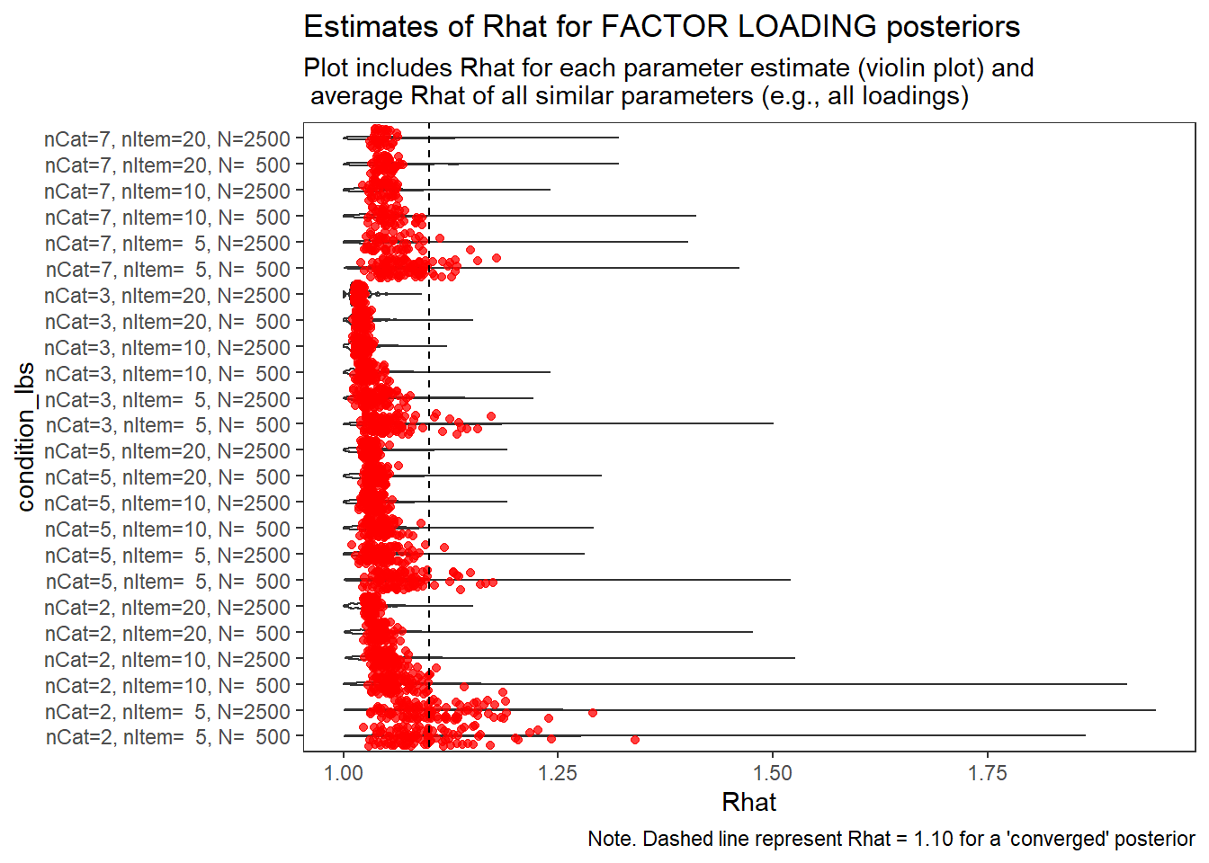
This is component of the project, a coarse grain investigation of the posteriors’ convergence will be assessed. In the proposal, I stated that I will evaluate convergence of the posteriors using the R-hat value as measures of convergence. R-hat values close to 1, within 0.1, will be considered a “converged” posterior for the parameter.

The code below loops through the posterior summaries to identify converged solutions.

mydata <- mydata %>%
  # group by condition, iteration, and parameter group to get Rhat more summarised
  group_by(condition, iter, parameter_group) %>%
  mutate(Rhat_paragrp = mean(Rhat)) %>%
  ungroup() %>%
  mutate(
    converge = ifelse(Rhat - 1.10 < 0, 1, 0),
    converge_paragrp = ifelse(Rhat_paragrp - 1.10 < 0, 1, 0)
  ) %>%
  group_by(condition, iter, parameter_group) %>%
  mutate(
     converge_proportion_paragrp = sum(converge)/n(),
  )

# Update condition labels for plotting
mydata$condition_lbs <- factor(
  mydata$condition, 
  levels = 1:24,
  labels = c(
    "nCat=2, nItem=  5, N=  500",
    "nCat=2, nItem=  5, N=2500",
    "nCat=2, nItem=10, N=  500",
    "nCat=2, nItem=10, N=2500",
    "nCat=2, nItem=20, N=  500",
    "nCat=2, nItem=20, N=2500",
    "nCat=5, nItem=  5, N=  500",
    "nCat=5, nItem=  5, N=2500",
    "nCat=5, nItem=10, N=  500",
    "nCat=5, nItem=10, N=2500",
    "nCat=5, nItem=20, N=  500",
    "nCat=5, nItem=20, N=2500",
    "nCat=3, nItem=  5, N=  500",
    "nCat=3, nItem=  5, N=2500",
    "nCat=3, nItem=10, N=  500",
    "nCat=3, nItem=10, N=2500",
    "nCat=3, nItem=20, N=  500",
    "nCat=3, nItem=20, N=2500",
    "nCat=7, nItem=  5, N=  500",
    "nCat=7, nItem=  5, N=2500",
    "nCat=7, nItem=10, N=  500",
    "nCat=7, nItem=10, N=2500",
    "nCat=7, nItem=20, N=  500",
    "nCat=7, nItem=20, N=2500"
  )
)

# columns to keep
keep_cols <- c("condition","condition_lbs", "iter", "N", "N_items", "N_cat", "parameter_group", "Rhat_paragrp", "converge_paragrp")

Summaring Convergence

Factor Loadings (\(\lambda\))

param = "FACTOR LOADING"

conv <- mydata %>%
  filter(parameter_group == "lambda")

conv_para_grp <- mydata %>%
  filter(parameter_group == "lambda") %>%
  select(all_of(keep_cols)) %>%
  distinct()

# tabular summary
conv_tbl <- conv %>%
  group_by(condition, N_cat, N_items, N) %>%
  summarise(Max_Converged=n(),
            Obs_Converged=sum(converge),
            Prop_Converged=Obs_Converged/Max_Converged)

`summarise()` has grouped output by 'condition', 'N_cat', 'N_items'. You can override using the `.groups` argument.

kable(conv_tbl, format="html", digits=3) %>%
  kable_styling(full_width = T)

condition	N_cat	N_items	N	Max_Converged	Obs_Converged	Prop_Converged
1	2	5	500	500	341	0.682
2	2	5	2500	500	327	0.654
3	2	10	500	1000	846	0.846
4	2	10	2500	1000	900	0.900
5	2	20	500	2000	1898	0.949
6	2	20	2500	2000	1945	0.973
7	5	5	500	500	388	0.776
8	5	5	2500	500	456	0.912
9	5	10	500	1000	920	0.920
10	5	10	2500	1000	965	0.965
11	5	20	500	2000	1890	0.945
12	5	20	2500	2000	1933	0.967
13	3	5	500	500	433	0.866
14	3	5	2500	500	474	0.948
15	3	10	500	1000	980	0.980
16	3	10	2500	1000	995	0.995
17	3	20	500	2000	1987	0.994
18	3	20	2500	2000	2000	1.000
19	7	5	500	500	389	0.778
20	7	5	2500	250	207	0.828
21	7	10	500	500	424	0.848
22	7	10	2500	500	451	0.902
23	7	20	500	1000	879	0.879
24	7	20	2500	760	700	0.921

conv_grp_tbl <- conv_para_grp %>%
  group_by(condition, N_cat, N_items, N) %>%
  summarise(Max_Converged=n(),
            Obs_Converged=sum(converge_paragrp),
            Prop_Converged=Obs_Converged/Max_Converged)

`summarise()` has grouped output by 'condition', 'N_cat', 'N_items'. You can override using the `.groups` argument.

kable(conv_grp_tbl, format="html", digits=3) %>%
  kable_styling(full_width = T)

condition	N_cat	N_items	N	Max_Converged	Obs_Converged	Prop_Converged
1	2	5	500	100	69	0.69
2	2	5	2500	100	56	0.56
3	2	10	500	100	97	0.97
4	2	10	2500	100	99	0.99
5	2	20	500	100	100	1.00
6	2	20	2500	100	100	1.00
7	5	5	500	100	89	0.89
8	5	5	2500	100	99	0.99
9	5	10	500	100	100	1.00
10	5	10	2500	100	100	1.00
11	5	20	500	100	100	1.00
12	5	20	2500	100	100	1.00
13	3	5	500	100	90	0.90
14	3	5	2500	100	100	1.00
15	3	10	500	100	100	1.00
16	3	10	2500	100	100	1.00
17	3	20	500	100	100	1.00
18	3	20	2500	100	100	1.00
19	7	5	500	100	87	0.87
20	7	5	2500	50	48	0.96
21	7	10	500	50	50	1.00
22	7	10	2500	50	50	1.00
23	7	20	500	50	50	1.00
24	7	20	2500	38	38	1.00

# visualize Rhat values
conv_grp <- conv %>%
  select(condition_lbs, iter, N_cat, N_items, N, Rhat_paragrp, converge_paragrp) %>%
  distinct()

Adding missing grouping variables: `condition`, `parameter_group`

ggplot() +
  geom_violin(data=conv, aes(x=condition_lbs , y=Rhat, group=condition))+
  geom_jitter(data=conv_grp, aes(x=condition_lbs , y=Rhat_paragrp), color="red", alpha=0.75)+
  geom_abline(intercept = 1.10, slope=0, linetype="dashed")+
  coord_flip()+
  labs(
    title=paste0("Estimates of Rhat for ", param, " posteriors" ),
    subtitle ="Plot includes Rhat for each parameter estimate (violin plot) and\n average Rhat of all similar parameters (e.g., all loadings)",
    caption = "Note. Dashed line represent Rhat = 1.10 for a 'converged' posterior"
  ) +
  theme_bw()+
  theme(
    panel.grid = element_blank()
  )

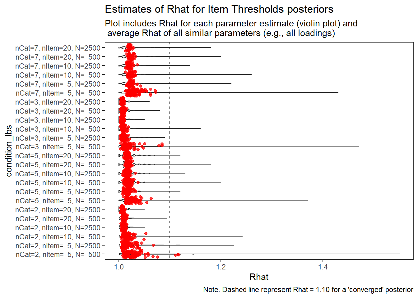
Item Thresholds (\(\tau\))

param = "Item Thresholds"

conv <- mydata %>%
  filter(parameter_group == "tau")

conv_para_grp <- mydata %>%
  filter(parameter_group == "tau") %>%
  select(all_of(keep_cols)) %>%
  distinct()

# tabular summary
conv_tbl <- conv %>%
  group_by(condition, N_cat, N_items, N) %>%
  summarise(Max_Converged=n(),
            Obs_Converged=sum(converge),
            Prop_Converged=Obs_Converged/Max_Converged)

`summarise()` has grouped output by 'condition', 'N_cat', 'N_items'. You can override using the `.groups` argument.

kable(conv_tbl, format="html", digits=3) %>%
  kable_styling(full_width = T)

condition	N_cat	N_items	N	Max_Converged	Obs_Converged	Prop_Converged
1	2	5	500	500	478	0.956
2	2	5	2500	500	491	0.982
3	2	10	500	1000	985	0.985
4	2	10	2500	1000	1000	1.000
5	2	20	500	2000	2000	1.000
6	2	20	2500	2000	2000	1.000
7	5	5	500	2000	1943	0.972
8	5	5	2500	2000	1997	0.999
9	5	10	500	4000	3980	0.995
10	5	10	2500	4000	3998	1.000
11	5	20	500	8000	7970	0.996
12	5	20	2500	8000	7990	0.999
13	3	5	500	1000	977	0.977
14	3	5	2500	1000	1000	1.000
15	3	10	500	2000	1997	0.999
16	3	10	2500	2000	2000	1.000
17	3	20	500	4000	4000	1.000
18	3	20	2500	4000	4000	1.000
19	7	5	500	3000	2854	0.951
20	7	5	2500	1500	1483	0.989
21	7	10	500	3000	2971	0.990
22	7	10	2500	3000	2989	0.996
23	7	20	500	6000	5933	0.989
24	7	20	2500	4560	4538	0.995

conv_grp_tbl <- conv_para_grp %>%
  group_by(condition, N_cat, N_items, N) %>%
  summarise(Max_Converged=n(),
            Obs_Converged=sum(converge_paragrp),
            Prop_Converged=Obs_Converged/Max_Converged)

`summarise()` has grouped output by 'condition', 'N_cat', 'N_items'. You can override using the `.groups` argument.

kable(conv_grp_tbl, format="html", digits=3) %>%
  kable_styling(full_width = T)

condition	N_cat	N_items	N	Max_Converged	Obs_Converged	Prop_Converged
1	2	5	500	100	97	0.97
2	2	5	2500	100	100	1.00
3	2	10	500	100	100	1.00
4	2	10	2500	100	100	1.00
5	2	20	500	100	100	1.00
6	2	20	2500	100	100	1.00
7	5	5	500	100	100	1.00
8	5	5	2500	100	100	1.00
9	5	10	500	100	100	1.00
10	5	10	2500	100	100	1.00
11	5	20	500	100	100	1.00
12	5	20	2500	100	100	1.00
13	3	5	500	100	100	1.00
14	3	5	2500	100	100	1.00
15	3	10	500	100	100	1.00
16	3	10	2500	100	100	1.00
17	3	20	500	100	100	1.00
18	3	20	2500	100	100	1.00
19	7	5	500	100	100	1.00
20	7	5	2500	50	50	1.00
21	7	10	500	50	50	1.00
22	7	10	2500	50	50	1.00
23	7	20	500	50	50	1.00
24	7	20	2500	38	38	1.00

# visualize Rhat values
conv_grp <- conv %>%
  select(condition_lbs, iter, N_cat, N_items, N, Rhat_paragrp, converge_paragrp) %>%
  distinct()

Adding missing grouping variables: `condition`, `parameter_group`

ggplot() +
  geom_violin(data=conv, aes(x=condition_lbs , y=Rhat, group=condition))+
  geom_jitter(data=conv_grp, aes(x=condition_lbs , y=Rhat_paragrp), color="red", alpha=0.75)+
  geom_abline(intercept = 1.10, slope=0, linetype="dashed")+
  coord_flip()+
  labs(
    title=paste0("Estimates of Rhat for ", param, " posteriors" ),
    subtitle ="Plot includes Rhat for each parameter estimate (violin plot) and\n average Rhat of all similar parameters (e.g., all loadings)",
    caption = "Note. Dashed line represent Rhat = 1.10 for a 'converged' posterior"
  ) +
  theme_bw()+
  theme(
    panel.grid = element_blank()
  )

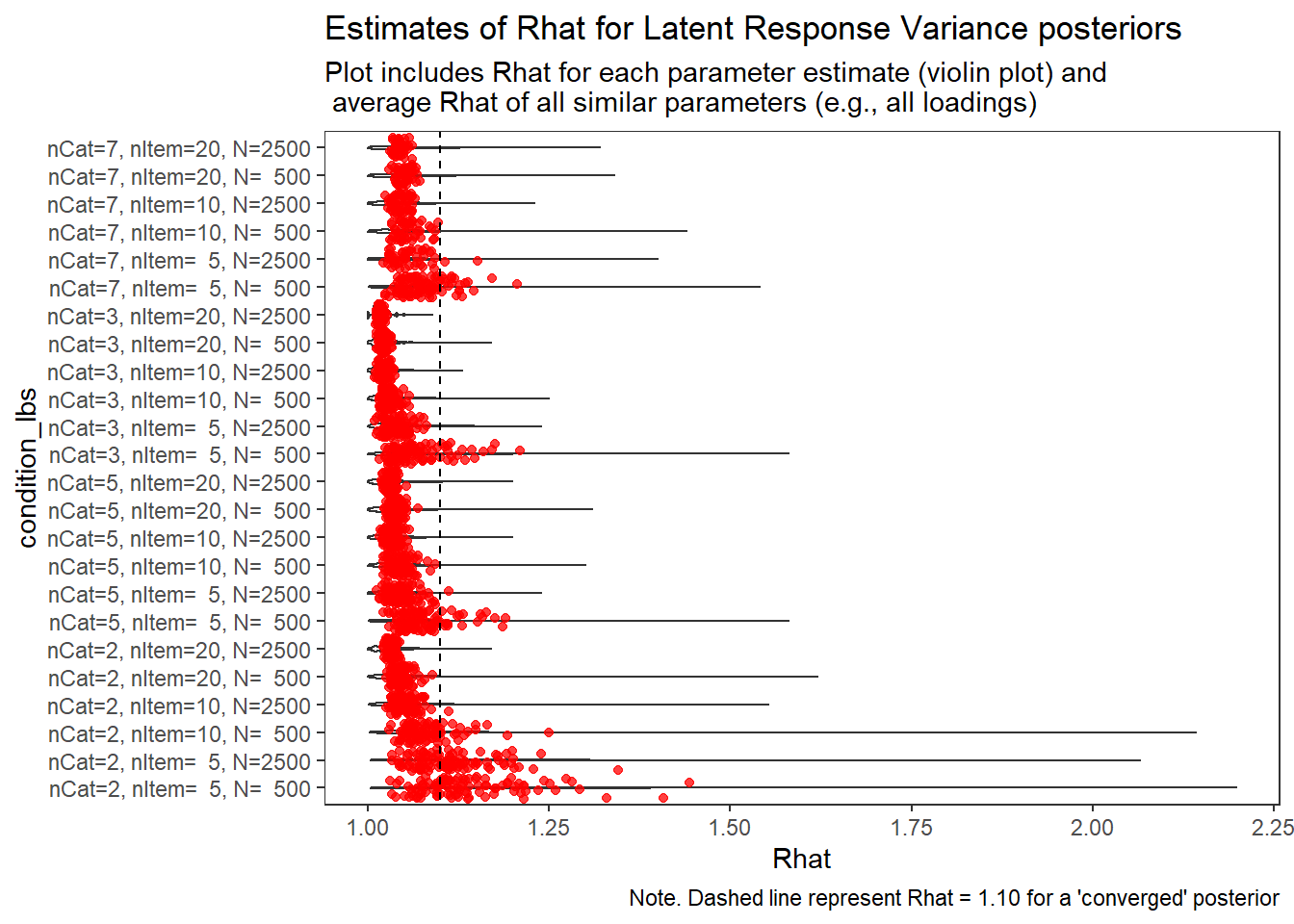
Latent Response Variance (\(\theta\))

param = "Latent Response Variance"

conv <- mydata %>%
  filter(parameter_group == "theta")

conv_para_grp <- mydata %>%
  filter(parameter_group == "theta") %>%
  select(all_of(keep_cols)) %>%
  distinct()

# tabular summary
conv_tbl <- conv %>%
  group_by(condition, N_cat, N_items, N) %>%
  summarise(Max_Converged=n(),
            Obs_Converged=sum(converge),
            Prop_Converged=Obs_Converged/Max_Converged)

`summarise()` has grouped output by 'condition', 'N_cat', 'N_items'. You can override using the `.groups` argument.

kable(conv_tbl, format="html", digits=3) %>%
  kable_styling(full_width = T)

condition	N_cat	N_items	N	Max_Converged	Obs_Converged	Prop_Converged
1	2	5	500	500	250	0.500
2	2	5	2500	500	310	0.620
3	2	10	500	1000	756	0.756
4	2	10	2500	1000	887	0.887
5	2	20	500	2000	1844	0.922
6	2	20	2500	2000	1941	0.971
7	5	5	500	500	366	0.732
8	5	5	2500	500	452	0.904
9	5	10	500	1000	908	0.908
10	5	10	2500	1000	964	0.964
11	5	20	500	2000	1876	0.938
12	5	20	2500	2000	1932	0.966
13	3	5	500	500	402	0.804
14	3	5	2500	500	465	0.930
15	3	10	500	1000	976	0.976
16	3	10	2500	1000	993	0.993
17	3	20	500	2000	1986	0.993
18	3	20	2500	2000	2000	1.000
19	7	5	500	500	374	0.748
20	7	5	2500	250	205	0.820
21	7	10	500	500	420	0.840
22	7	10	2500	500	451	0.902
23	7	20	500	1000	861	0.861
24	7	20	2500	760	700	0.921

conv_grp_tbl <- conv_para_grp %>%
  group_by(condition, N_cat, N_items, N) %>%
  summarise(Max_Converged=n(),
            Obs_Converged=sum(converge_paragrp),
            Prop_Converged=Obs_Converged/Max_Converged)

`summarise()` has grouped output by 'condition', 'N_cat', 'N_items'. You can override using the `.groups` argument.

kable(conv_grp_tbl, format="html", digits=3) %>%
  kable_styling(full_width = T)

condition	N_cat	N_items	N	Max_Converged	Obs_Converged	Prop_Converged
1	2	5	500	100	33	0.33
2	2	5	2500	100	46	0.46
3	2	10	500	100	85	0.85
4	2	10	2500	100	99	0.99
5	2	20	500	100	100	1.00
6	2	20	2500	100	100	1.00
7	5	5	500	100	82	0.82
8	5	5	2500	100	99	0.99
9	5	10	500	100	100	1.00
10	5	10	2500	100	100	1.00
11	5	20	500	100	100	1.00
12	5	20	2500	100	100	1.00
13	3	5	500	100	82	0.82
14	3	5	2500	100	100	1.00
15	3	10	500	100	100	1.00
16	3	10	2500	100	100	1.00
17	3	20	500	100	100	1.00
18	3	20	2500	100	100	1.00
19	7	5	500	100	79	0.79
20	7	5	2500	50	48	0.96
21	7	10	500	50	50	1.00
22	7	10	2500	50	50	1.00
23	7	20	500	50	50	1.00
24	7	20	2500	38	38	1.00

# visualize Rhat values
conv_grp <- conv %>%
  select(condition_lbs, iter, N_cat, N_items, N, Rhat_paragrp, converge_paragrp) %>%
  distinct()

Adding missing grouping variables: `condition`, `parameter_group`

ggplot() +
  geom_violin(data=conv, aes(x=condition_lbs , y=Rhat, group=condition))+
  geom_jitter(data=conv_grp, aes(x=condition_lbs , y=Rhat_paragrp), color="red", alpha=0.75)+
  geom_abline(intercept = 1.10, slope=0, linetype="dashed")+
  coord_flip()+
  labs(
    title=paste0("Estimates of Rhat for ", param, " posteriors" ),
    subtitle ="Plot includes Rhat for each parameter estimate (violin plot) and\n average Rhat of all similar parameters (e.g., all loadings)",
    caption = "Note. Dashed line represent Rhat = 1.10 for a 'converged' posterior"
  ) +
  theme_bw()+
  theme(
    panel.grid = element_blank()
  )

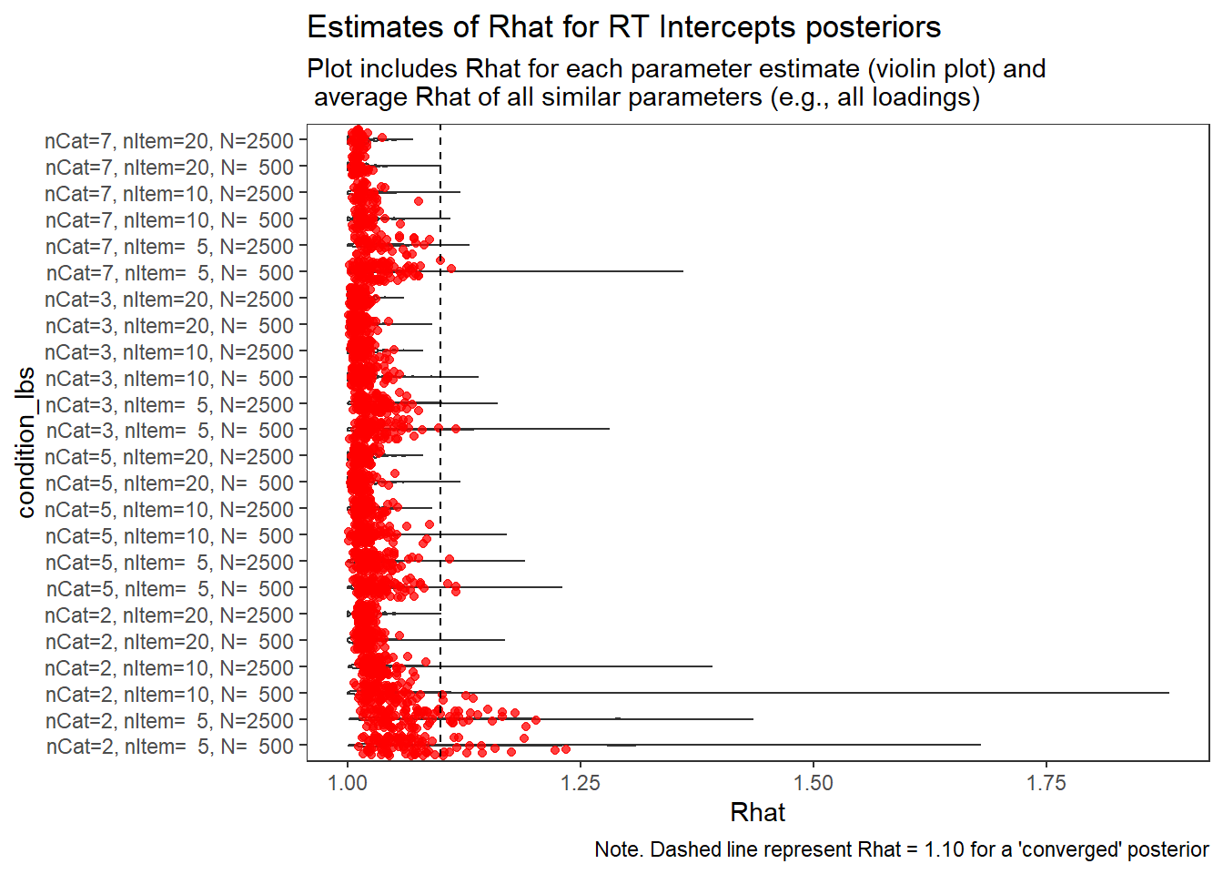
Response Time Intercepts (\(\beta_{lrt}\))

param = "RT Intercepts"

conv <- mydata %>%
  filter(parameter_group == "beta_lrt")

conv_para_grp <- mydata %>%
  filter(parameter_group == "beta_lrt") %>%
  select(all_of(keep_cols)) %>%
  distinct()

# tabular summary
conv_tbl <- conv %>%
  group_by(condition, N_cat, N_items, N) %>%
  summarise(Max_Converged=n(),
            Obs_Converged=sum(converge),
            Prop_Converged=Obs_Converged/Max_Converged)

`summarise()` has grouped output by 'condition', 'N_cat', 'N_items'. You can override using the `.groups` argument.

kable(conv_tbl, format="html", digits=3) %>%
  kable_styling(full_width = T)

condition	N_cat	N_items	N	Max_Converged	Obs_Converged	Prop_Converged
1	2	5	500	500	402	0.804
2	2	5	2500	500	401	0.802
3	2	10	500	1000	927	0.927
4	2	10	2500	1000	974	0.974
5	2	20	500	2000	1986	0.993
6	2	20	2500	2000	1999	1.000
7	5	5	500	500	464	0.928
8	5	5	2500	500	488	0.976
9	5	10	500	1000	984	0.984
10	5	10	2500	1000	1000	1.000
11	5	20	500	2000	1995	0.998
12	5	20	2500	2000	2000	1.000
13	3	5	500	500	480	0.960
14	3	5	2500	500	494	0.988
15	3	10	500	1000	996	0.996
16	3	10	2500	1000	1000	1.000
17	3	20	500	2000	2000	1.000
18	3	20	2500	2000	2000	1.000
19	7	5	500	500	482	0.964
20	7	5	2500	250	237	0.948
21	7	10	500	500	497	0.994
22	7	10	2500	500	497	0.994
23	7	20	500	1000	999	0.999
24	7	20	2500	760	760	1.000

conv_grp_tbl <- conv_para_grp %>%
  group_by(condition, N_cat, N_items, N) %>%
  summarise(Max_Converged=n(),
            Obs_Converged=sum(converge_paragrp),
            Prop_Converged=Obs_Converged/Max_Converged)

`summarise()` has grouped output by 'condition', 'N_cat', 'N_items'. You can override using the `.groups` argument.

kable(conv_grp_tbl, format="html", digits=3) %>%
  kable_styling(full_width = T)

condition	N_cat	N_items	N	Max_Converged	Obs_Converged	Prop_Converged
1	2	5	500	100	85	0.85
2	2	5	2500	100	81	0.81
3	2	10	500	100	96	0.96
4	2	10	2500	100	100	1.00
5	2	20	500	100	100	1.00
6	2	20	2500	100	100	1.00
7	5	5	500	100	97	0.97
8	5	5	2500	100	99	0.99
9	5	10	500	100	100	1.00
10	5	10	2500	100	100	1.00
11	5	20	500	100	100	1.00
12	5	20	2500	100	100	1.00
13	3	5	500	100	99	0.99
14	3	5	2500	100	100	1.00
15	3	10	500	100	100	1.00
16	3	10	2500	100	100	1.00
17	3	20	500	100	100	1.00
18	3	20	2500	100	100	1.00
19	7	5	500	100	98	0.98
20	7	5	2500	50	50	1.00
21	7	10	500	50	50	1.00
22	7	10	2500	50	50	1.00
23	7	20	500	50	50	1.00
24	7	20	2500	38	38	1.00

# visualize Rhat values
conv_grp <- conv %>%
  select(condition_lbs, iter, N_cat, N_items, N, Rhat_paragrp, converge_paragrp) %>%
  distinct()

Adding missing grouping variables: `condition`, `parameter_group`

ggplot() +
  geom_violin(data=conv, aes(x=condition_lbs , y=Rhat, group=condition))+
  geom_jitter(data=conv_grp, aes(x=condition_lbs , y=Rhat_paragrp), color="red", alpha=0.75)+
  geom_abline(intercept = 1.10, slope=0, linetype="dashed")+
  coord_flip()+
  labs(
    title=paste0("Estimates of Rhat for ", param, " posteriors" ),
    subtitle ="Plot includes Rhat for each parameter estimate (violin plot) and\n average Rhat of all similar parameters (e.g., all loadings)",
    caption = "Note. Dashed line represent Rhat = 1.10 for a 'converged' posterior"
  ) +
  theme_bw()+
  theme(
    panel.grid = element_blank()
  )

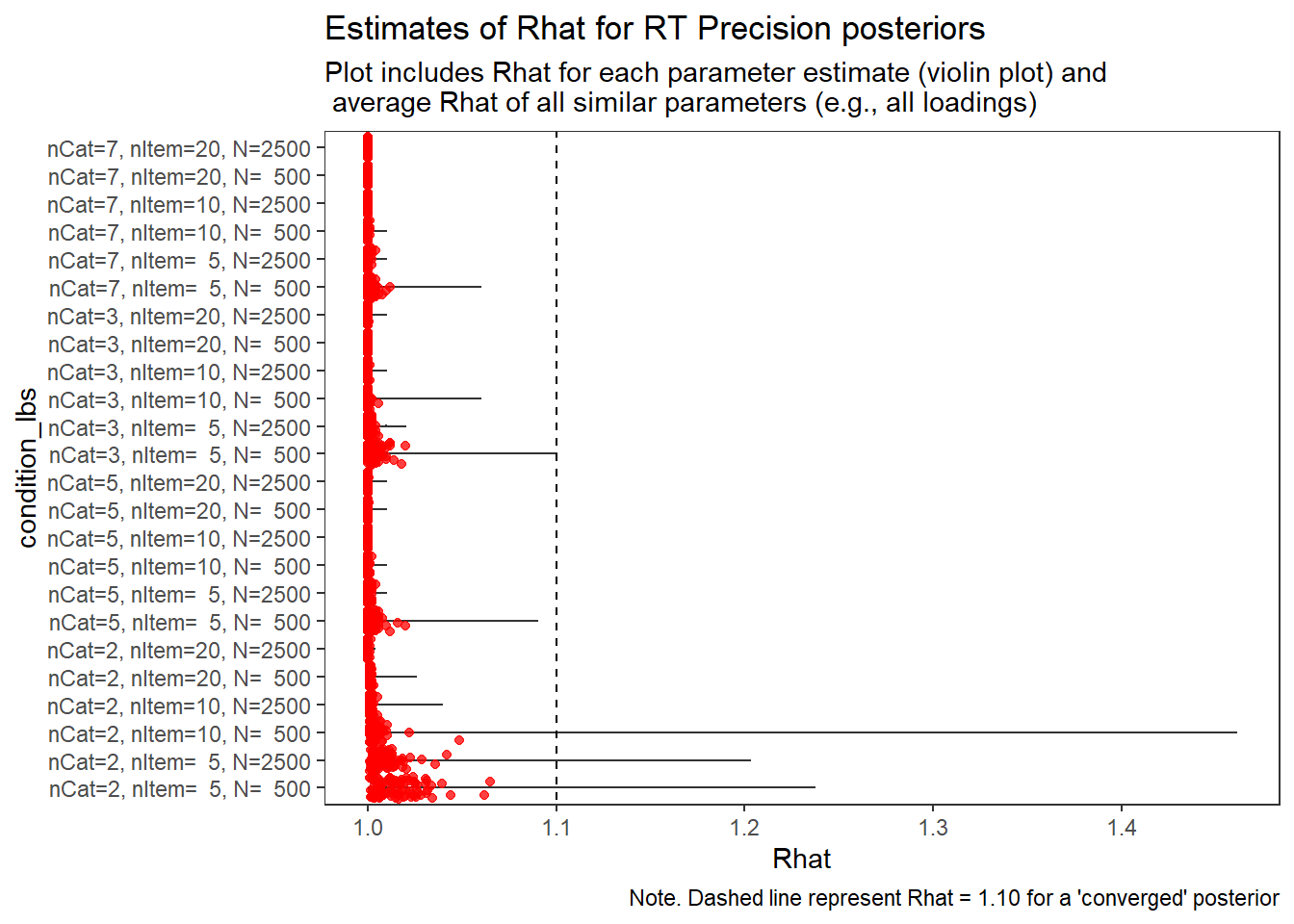
Response Time Precision (\(\sigma_{lrt}\))

param = "RT Precision"

conv <- mydata %>%
  filter(parameter_group == "sigma_lrt")

conv_para_grp <- mydata %>%
  filter(parameter_group == "sigma_lrt") %>%
  select(all_of(keep_cols)) %>%
  distinct()

# tabular summary
conv_tbl <- conv %>%
  group_by(condition, N_cat, N_items, N) %>%
  summarise(Max_Converged=n(),
            Obs_Converged=sum(converge),
            Prop_Converged=Obs_Converged/Max_Converged)

`summarise()` has grouped output by 'condition', 'N_cat', 'N_items'. You can override using the `.groups` argument.

kable(conv_tbl, format="html", digits=3) %>%
  kable_styling(full_width = T)

condition	N_cat	N_items	N	Max_Converged	Obs_Converged	Prop_Converged
1	2	5	500	500	485	0.970
2	2	5	2500	500	497	0.994
3	2	10	500	1000	998	0.998
4	2	10	2500	1000	1000	1.000
5	2	20	500	2000	2000	1.000
6	2	20	2500	2000	2000	1.000
7	5	5	500	500	500	1.000
8	5	5	2500	500	500	1.000
9	5	10	500	1000	1000	1.000
10	5	10	2500	1000	1000	1.000
11	5	20	500	2000	2000	1.000
12	5	20	2500	2000	2000	1.000
13	3	5	500	500	499	0.998
14	3	5	2500	500	500	1.000
15	3	10	500	1000	1000	1.000
16	3	10	2500	1000	1000	1.000
17	3	20	500	2000	2000	1.000
18	3	20	2500	2000	2000	1.000
19	7	5	500	500	500	1.000
20	7	5	2500	250	250	1.000
21	7	10	500	500	500	1.000
22	7	10	2500	500	500	1.000
23	7	20	500	1000	1000	1.000
24	7	20	2500	760	760	1.000

conv_grp_tbl <- conv_para_grp %>%
  group_by(condition, N_cat, N_items, N) %>%
  summarise(Max_Converged=n(),
            Obs_Converged=sum(converge_paragrp),
            Prop_Converged=Obs_Converged/Max_Converged)

`summarise()` has grouped output by 'condition', 'N_cat', 'N_items'. You can override using the `.groups` argument.

kable(conv_grp_tbl, format="html", digits=3) %>%
  kable_styling(full_width = T)

condition	N_cat	N_items	N	Max_Converged	Obs_Converged	Prop_Converged
1	2	5	500	100	100	1
2	2	5	2500	100	100	1
3	2	10	500	100	100	1
4	2	10	2500	100	100	1
5	2	20	500	100	100	1
6	2	20	2500	100	100	1
7	5	5	500	100	100	1
8	5	5	2500	100	100	1
9	5	10	500	100	100	1
10	5	10	2500	100	100	1
11	5	20	500	100	100	1
12	5	20	2500	100	100	1
13	3	5	500	100	100	1
14	3	5	2500	100	100	1
15	3	10	500	100	100	1
16	3	10	2500	100	100	1
17	3	20	500	100	100	1
18	3	20	2500	100	100	1
19	7	5	500	100	100	1
20	7	5	2500	50	50	1
21	7	10	500	50	50	1
22	7	10	2500	50	50	1
23	7	20	500	50	50	1
24	7	20	2500	38	38	1

# visualize Rhat values
conv_grp <- conv %>%
  select(condition_lbs, iter, N_cat, N_items, N, Rhat_paragrp, converge_paragrp) %>%
  distinct()

Adding missing grouping variables: `condition`, `parameter_group`

ggplot() +
  geom_violin(data=conv, aes(x=condition_lbs , y=Rhat, group=condition))+
  geom_jitter(data=conv_grp, aes(x=condition_lbs , y=Rhat_paragrp), color="red", alpha=0.75)+
  geom_abline(intercept = 1.10, slope=0, linetype="dashed")+
  coord_flip()+
  labs(
    title=paste0("Estimates of Rhat for ", param, " posteriors" ),
    subtitle ="Plot includes Rhat for each parameter estimate (violin plot) and\n average Rhat of all similar parameters (e.g., all loadings)",
    caption = "Note. Dashed line represent Rhat = 1.10 for a 'converged' posterior"
  ) +
  theme_bw()+
  theme(
    panel.grid = element_blank()
  )

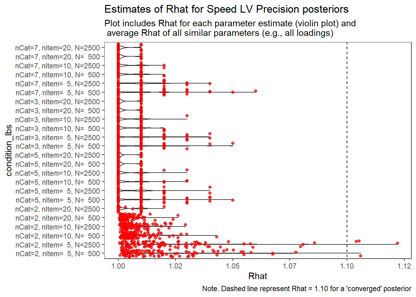
Response Time Factor Precision (\(\sigma_s\))

param = "Speed LV Precision"

conv <- mydata %>%
  filter(parameter_group == "sigma_s")

conv_para_grp <- mydata %>%
  filter(parameter_group == "sigma_s") %>%
  select(all_of(keep_cols)) %>%
  distinct()

# tabular summary
conv_tbl <- conv %>%
  group_by(condition, N_cat, N_items, N) %>%
  summarise(Max_Converged=n(),
            Obs_Converged=sum(converge),
            Prop_Converged=Obs_Converged/Max_Converged)

`summarise()` has grouped output by 'condition', 'N_cat', 'N_items'. You can override using the `.groups` argument.

kable(conv_tbl, format="html", digits=3) %>%
  kable_styling(full_width = T)

condition	N_cat	N_items	N	Max_Converged	Obs_Converged	Prop_Converged
1	2	5	500	100	99	0.99
2	2	5	2500	100	97	0.97
3	2	10	500	100	100	1.00
4	2	10	2500	100	100	1.00
5	2	20	500	100	100	1.00
6	2	20	2500	100	100	1.00
7	5	5	500	100	100	1.00
8	5	5	2500	100	100	1.00
9	5	10	500	100	100	1.00
10	5	10	2500	100	100	1.00
11	5	20	500	100	100	1.00
12	5	20	2500	100	100	1.00
13	3	5	500	100	100	1.00
14	3	5	2500	100	100	1.00
15	3	10	500	100	100	1.00
16	3	10	2500	100	100	1.00
17	3	20	500	100	100	1.00
18	3	20	2500	100	100	1.00
19	7	5	500	100	100	1.00
20	7	5	2500	50	50	1.00
21	7	10	500	50	50	1.00
22	7	10	2500	50	50	1.00
23	7	20	500	50	50	1.00
24	7	20	2500	38	38	1.00

conv_grp_tbl <- conv_para_grp %>%
  group_by(condition, N_cat, N_items, N) %>%
  summarise(Max_Converged=n(),
            Obs_Converged=sum(converge_paragrp),
            Prop_Converged=Obs_Converged/Max_Converged)

`summarise()` has grouped output by 'condition', 'N_cat', 'N_items'. You can override using the `.groups` argument.

kable(conv_grp_tbl, format="html", digits=3) %>%
  kable_styling(full_width = T)

condition	N_cat	N_items	N	Max_Converged	Obs_Converged	Prop_Converged
1	2	5	500	100	99	0.99
2	2	5	2500	100	97	0.97
3	2	10	500	100	100	1.00
4	2	10	2500	100	100	1.00
5	2	20	500	100	100	1.00
6	2	20	2500	100	100	1.00
7	5	5	500	100	100	1.00
8	5	5	2500	100	100	1.00
9	5	10	500	100	100	1.00
10	5	10	2500	100	100	1.00
11	5	20	500	100	100	1.00
12	5	20	2500	100	100	1.00
13	3	5	500	100	100	1.00
14	3	5	2500	100	100	1.00
15	3	10	500	100	100	1.00
16	3	10	2500	100	100	1.00
17	3	20	500	100	100	1.00
18	3	20	2500	100	100	1.00
19	7	5	500	100	100	1.00
20	7	5	2500	50	50	1.00
21	7	10	500	50	50	1.00
22	7	10	2500	50	50	1.00
23	7	20	500	50	50	1.00
24	7	20	2500	38	38	1.00

# visualize Rhat values
conv_grp <- conv %>%
  select(condition_lbs, iter, N_cat, N_items, N, Rhat_paragrp, converge_paragrp) %>%
  distinct()

Adding missing grouping variables: `condition`, `parameter_group`

ggplot() +
  geom_violin(data=conv, aes(x=condition_lbs , y=Rhat, group=condition))+
  geom_jitter(data=conv_grp, aes(x=condition_lbs , y=Rhat_paragrp), color="red", alpha=0.75)+
  geom_abline(intercept = 1.10, slope=0, linetype="dashed")+
  coord_flip()+
  labs(
    title=paste0("Estimates of Rhat for ", param, " posteriors" ),
    subtitle ="Plot includes Rhat for each parameter estimate (violin plot) and\n average Rhat of all similar parameters (e.g., all loadings)",
    caption = "Note. Dashed line represent Rhat = 1.10 for a 'converged' posterior"
  ) +
  theme_bw()+
  theme(
    panel.grid = element_blank()
  )

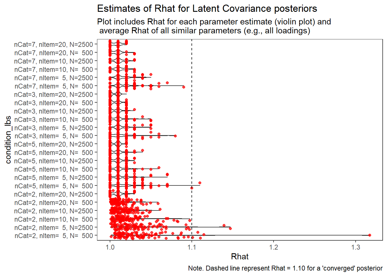
Factor Covariance (\(\sigma_{st}\))

param = "Latent Covariance"

conv <- mydata %>%
  filter(parameter_group == "sigma_st")

conv_para_grp <- mydata %>%
  filter(parameter_group == "sigma_st") %>%
  select(all_of(keep_cols)) %>%
  distinct()

# tabular summary
conv_tbl <- conv %>%
  group_by(condition, N_cat, N_items, N) %>%
  summarise(Max_Converged=n(),
            Obs_Converged=sum(converge),
            Prop_Converged=Obs_Converged/Max_Converged)

`summarise()` has grouped output by 'condition', 'N_cat', 'N_items'. You can override using the `.groups` argument.

kable(conv_tbl, format="html", digits=3) %>%
  kable_styling(full_width = T)

condition	N_cat	N_items	N	Max_Converged	Obs_Converged	Prop_Converged
1	2	5	500	100	95	0.95
2	2	5	2500	100	98	0.98
3	2	10	500	100	100	1.00
4	2	10	2500	100	100	1.00
5	2	20	500	100	100	1.00
6	2	20	2500	100	100	1.00
7	5	5	500	100	98	0.98
8	5	5	2500	100	100	1.00
9	5	10	500	100	100	1.00
10	5	10	2500	100	100	1.00
11	5	20	500	100	100	1.00
12	5	20	2500	100	100	1.00
13	3	5	500	100	100	1.00
14	3	5	2500	100	100	1.00
15	3	10	500	100	100	1.00
16	3	10	2500	100	100	1.00
17	3	20	500	100	100	1.00
18	3	20	2500	100	100	1.00
19	7	5	500	100	100	1.00
20	7	5	2500	50	50	1.00
21	7	10	500	50	50	1.00
22	7	10	2500	50	50	1.00
23	7	20	500	50	50	1.00
24	7	20	2500	38	38	1.00

conv_grp_tbl <- conv_para_grp %>%
  group_by(condition, N_cat, N_items, N) %>%
  summarise(Max_Converged=n(),
            Obs_Converged=sum(converge_paragrp),
            Prop_Converged=Obs_Converged/Max_Converged)

`summarise()` has grouped output by 'condition', 'N_cat', 'N_items'. You can override using the `.groups` argument.

kable(conv_grp_tbl, format="html", digits=3) %>%
  kable_styling(full_width = T)

condition	N_cat	N_items	N	Max_Converged	Obs_Converged	Prop_Converged
1	2	5	500	100	95	0.95
2	2	5	2500	100	98	0.98
3	2	10	500	100	100	1.00
4	2	10	2500	100	100	1.00
5	2	20	500	100	100	1.00
6	2	20	2500	100	100	1.00
7	5	5	500	100	98	0.98
8	5	5	2500	100	100	1.00
9	5	10	500	100	100	1.00
10	5	10	2500	100	100	1.00
11	5	20	500	100	100	1.00
12	5	20	2500	100	100	1.00
13	3	5	500	100	100	1.00
14	3	5	2500	100	100	1.00
15	3	10	500	100	100	1.00
16	3	10	2500	100	100	1.00
17	3	20	500	100	100	1.00
18	3	20	2500	100	100	1.00
19	7	5	500	100	100	1.00
20	7	5	2500	50	50	1.00
21	7	10	500	50	50	1.00
22	7	10	2500	50	50	1.00
23	7	20	500	50	50	1.00
24	7	20	2500	38	38	1.00

# visualize Rhat values
conv_grp <- conv %>%
  select(condition_lbs, iter, N_cat, N_items, N, Rhat_paragrp, converge_paragrp) %>%
  distinct()

Adding missing grouping variables: `condition`, `parameter_group`

ggplot() +
  geom_violin(data=conv, aes(x=condition_lbs , y=Rhat, group=condition))+
  geom_jitter(data=conv_grp, aes(x=condition_lbs , y=Rhat_paragrp), color="red", alpha=0.75)+
  geom_abline(intercept = 1.10, slope=0, linetype="dashed")+
  coord_flip()+
  labs(
    title=paste0("Estimates of Rhat for ", param, " posteriors" ),
    subtitle ="Plot includes Rhat for each parameter estimate (violin plot) and\n average Rhat of all similar parameters (e.g., all loadings)",
    caption = "Note. Dashed line represent Rhat = 1.10 for a 'converged' posterior"
  ) +
  theme_bw()+
  theme(
    panel.grid = element_blank()
  )

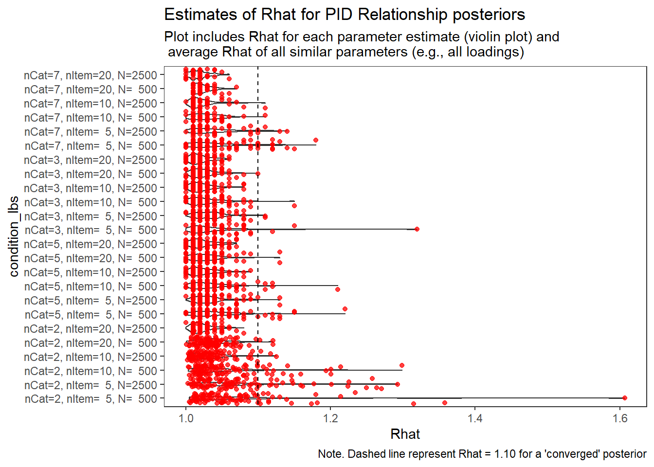
PID Relationship (\(\rho\))

param = "PID Relationship"

conv <- mydata %>%
  filter(parameter_group == "rho")

conv_para_grp <- mydata %>%
  filter(parameter_group == "rho") %>%
  select(all_of(keep_cols)) %>%
  distinct()

# tabular summary
conv_tbl <- conv %>%
  group_by(condition, N_cat, N_items, N) %>%
  summarise(Max_Converged=n(),
            Obs_Converged=sum(converge),
            Prop_Converged=Obs_Converged/Max_Converged)

`summarise()` has grouped output by 'condition', 'N_cat', 'N_items'. You can override using the `.groups` argument.

kable(conv_tbl, format="html", digits=3) %>%
  kable_styling(full_width = T)

condition	N_cat	N_items	N	Max_Converged	Obs_Converged	Prop_Converged
1	2	5	500	100	82	0.82
2	2	5	2500	100	80	0.80
3	2	10	500	100	85	0.85
4	2	10	2500	100	97	0.97
5	2	20	500	100	97	0.97
6	2	20	2500	100	100	1.00
7	5	5	500	100	91	0.91
8	5	5	2500	100	97	0.97
9	5	10	500	100	94	0.94
10	5	10	2500	100	100	1.00
11	5	20	500	100	98	0.98
12	5	20	2500	100	100	1.00
13	3	5	500	100	97	0.97
14	3	5	2500	100	98	0.98
15	3	10	500	100	99	0.99
16	3	10	2500	100	100	1.00
17	3	20	500	100	99	0.99
18	3	20	2500	100	100	1.00
19	7	5	500	100	87	0.87
20	7	5	2500	50	45	0.90
21	7	10	500	50	49	0.98
22	7	10	2500	50	49	0.98
23	7	20	500	50	50	1.00
24	7	20	2500	38	38	1.00

conv_grp_tbl <- conv_para_grp %>%
  group_by(condition, N_cat, N_items, N) %>%
  summarise(Max_Converged=n(),
            Obs_Converged=sum(converge_paragrp),
            Prop_Converged=Obs_Converged/Max_Converged)

`summarise()` has grouped output by 'condition', 'N_cat', 'N_items'. You can override using the `.groups` argument.

kable(conv_grp_tbl, format="html", digits=3) %>%
  kable_styling(full_width = T)

condition	N_cat	N_items	N	Max_Converged	Obs_Converged	Prop_Converged
1	2	5	500	100	82	0.82
2	2	5	2500	100	80	0.80
3	2	10	500	100	85	0.85
4	2	10	2500	100	97	0.97
5	2	20	500	100	97	0.97
6	2	20	2500	100	100	1.00
7	5	5	500	100	91	0.91
8	5	5	2500	100	97	0.97
9	5	10	500	100	94	0.94
10	5	10	2500	100	100	1.00
11	5	20	500	100	98	0.98
12	5	20	2500	100	100	1.00
13	3	5	500	100	97	0.97
14	3	5	2500	100	98	0.98
15	3	10	500	100	99	0.99
16	3	10	2500	100	100	1.00
17	3	20	500	100	99	0.99
18	3	20	2500	100	100	1.00
19	7	5	500	100	87	0.87
20	7	5	2500	50	45	0.90
21	7	10	500	50	49	0.98
22	7	10	2500	50	49	0.98
23	7	20	500	50	50	1.00
24	7	20	2500	38	38	1.00

# visualize Rhat values
conv_grp <- conv %>%
  select(condition_lbs, iter, N_cat, N_items, N, Rhat_paragrp, converge_paragrp) %>%
  distinct()

Adding missing grouping variables: `condition`, `parameter_group`

ggplot() +
  geom_violin(data=conv, aes(x=condition_lbs , y=Rhat, group=condition))+
  geom_jitter(data=conv_grp, aes(x=condition_lbs , y=Rhat_paragrp), color="red", alpha=0.75)+
  geom_abline(intercept = 1.10, slope=0, linetype="dashed")+
  coord_flip()+
  labs(
    title=paste0("Estimates of Rhat for ", param, " posteriors" ),
    subtitle ="Plot includes Rhat for each parameter estimate (violin plot) and\n average Rhat of all similar parameters (e.g., all loadings)",
    caption = "Note. Dashed line represent Rhat = 1.10 for a 'converged' posterior"
  ) +
  theme_bw()+
  theme(
    panel.grid = element_blank()
  )

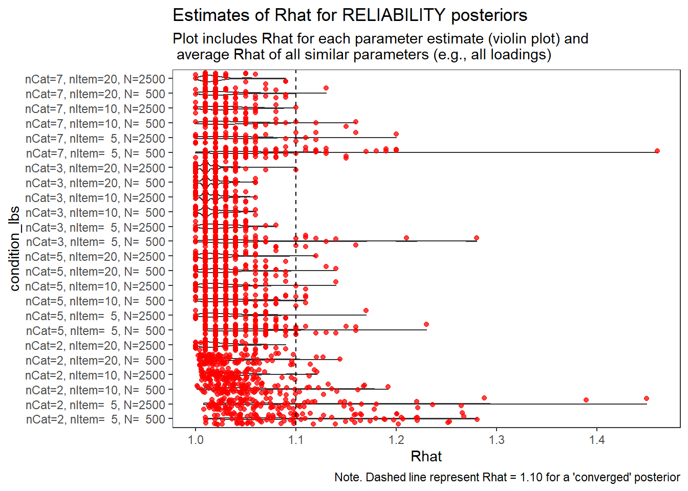
Factor Reliability (\(\omega\))

param = "RELIABILITY"

conv <- mydata %>%
  filter(parameter_group == "omega")

conv_para_grp <- mydata %>%
  filter(parameter_group == "omega") %>%
  select(all_of(keep_cols)) %>%
  distinct()

# tabular summary
conv_tbl <- conv %>%
  group_by(condition, N_cat, N_items, N) %>%
  summarise(Max_Converged=n(),
            Obs_Converged=sum(converge),
            Prop_Converged=Obs_Converged/Max_Converged)

`summarise()` has grouped output by 'condition', 'N_cat', 'N_items'. You can override using the `.groups` argument.

kable(conv_tbl, format="html", digits=3) %>%
  kable_styling(full_width = T)

condition	N_cat	N_items	N	Max_Converged	Obs_Converged	Prop_Converged
1	2	5	500	100	63	0.63
2	2	5	2500	100	78	0.78
3	2	10	500	100	88	0.88
4	2	10	2500	100	97	0.97
5	2	20	500	100	96	0.96
6	2	20	2500	100	100	1.00
7	5	5	500	100	87	0.87
8	5	5	2500	100	99	0.99
9	5	10	500	100	95	0.95
10	5	10	2500	100	97	0.97
11	5	20	500	100	98	0.98
12	5	20	2500	100	99	0.99
13	3	5	500	100	89	0.89
14	3	5	2500	100	100	1.00
15	3	10	500	100	100	1.00
16	3	10	2500	100	100	1.00
17	3	20	500	100	100	1.00
18	3	20	2500	100	99	0.99
19	7	5	500	100	81	0.81
20	7	5	2500	50	43	0.86
21	7	10	500	50	46	0.92
22	7	10	2500	50	49	0.98
23	7	20	500	50	49	0.98
24	7	20	2500	38	38	1.00

conv_grp_tbl <- conv_para_grp %>%
  group_by(condition, N_cat, N_items, N) %>%
  summarise(Max_Converged=n(),
            Obs_Converged=sum(converge_paragrp),
            Prop_Converged=Obs_Converged/Max_Converged)

`summarise()` has grouped output by 'condition', 'N_cat', 'N_items'. You can override using the `.groups` argument.

kable(conv_grp_tbl, format="html", digits=3) %>%
  kable_styling(full_width = T)

condition	N_cat	N_items	N	Max_Converged	Obs_Converged	Prop_Converged
1	2	5	500	100	63	0.63
2	2	5	2500	100	78	0.78
3	2	10	500	100	88	0.88
4	2	10	2500	100	97	0.97
5	2	20	500	100	96	0.96
6	2	20	2500	100	100	1.00
7	5	5	500	100	87	0.87
8	5	5	2500	100	99	0.99
9	5	10	500	100	95	0.95
10	5	10	2500	100	97	0.97
11	5	20	500	100	98	0.98
12	5	20	2500	100	99	0.99
13	3	5	500	100	89	0.89
14	3	5	2500	100	100	1.00
15	3	10	500	100	100	1.00
16	3	10	2500	100	100	1.00
17	3	20	500	100	100	1.00
18	3	20	2500	100	99	0.99
19	7	5	500	100	81	0.81
20	7	5	2500	50	43	0.86
21	7	10	500	50	46	0.92
22	7	10	2500	50	49	0.98
23	7	20	500	50	49	0.98
24	7	20	2500	38	38	1.00

# visualize Rhat values
conv_grp <- conv %>%
  select(condition_lbs, iter, N_cat, N_items, N, Rhat_paragrp, converge_paragrp) %>%
  distinct()

Adding missing grouping variables: `condition`, `parameter_group`

ggplot() +
  geom_violin(data=conv, aes(x=condition_lbs , y=Rhat, group=condition))+
  geom_jitter(data=conv_grp, aes(x=condition_lbs , y=Rhat_paragrp), color="red", alpha=0.75)+
  geom_abline(intercept = 1.10, slope=0, linetype="dashed")+
  coord_flip()+
  labs(
    title=paste0("Estimates of Rhat for ", param, " posteriors" ),
    subtitle ="Plot includes Rhat for each parameter estimate (violin plot) and\n average Rhat of all similar parameters (e.g., all loadings)",
    caption = "Note. Dashed line represent Rhat = 1.10 for a 'converged' posterior"
  ) +
  theme_bw()+
  theme(
    panel.grid = element_blank()
  )

Effect of Simulated Conditions

Factor Loadings (\(\lambda\))

conv_para_grp <- mydata %>%
  filter(parameter_group == "lambda") %>%
  select(all_of(keep_cols)) %>%
  distinct()

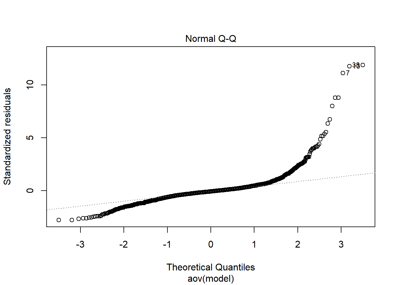
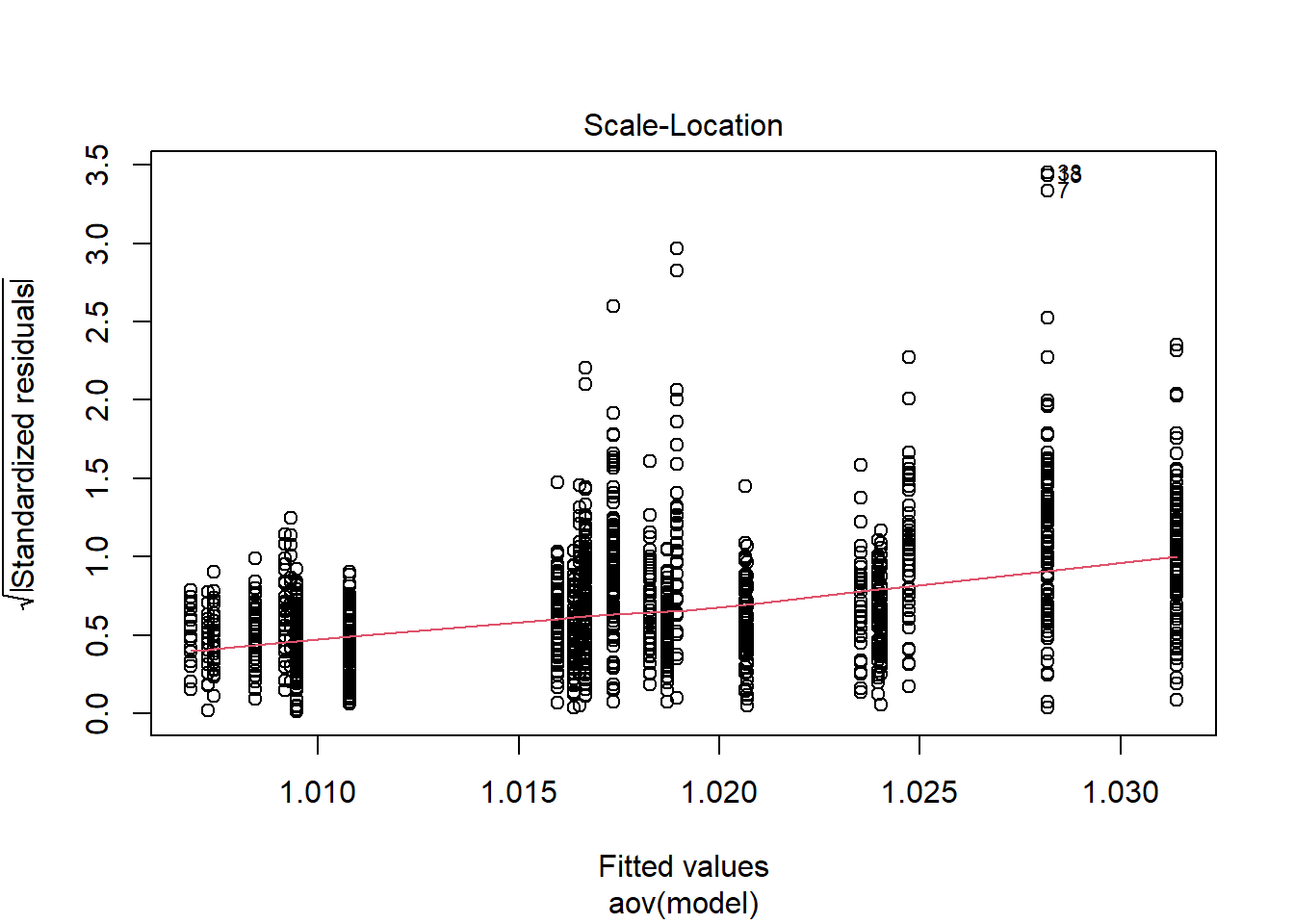
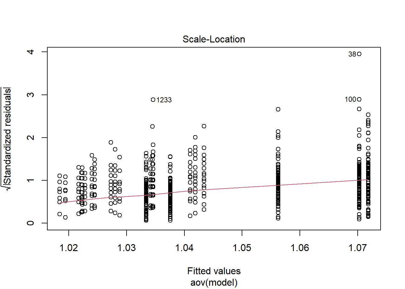
## ANOVA on Rhat values
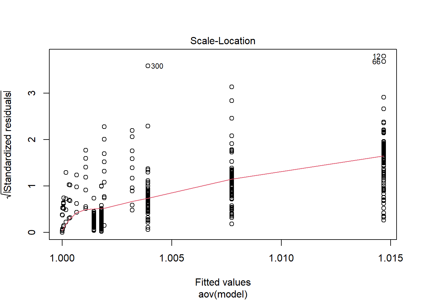
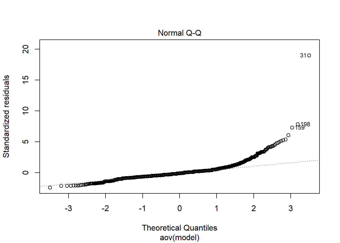
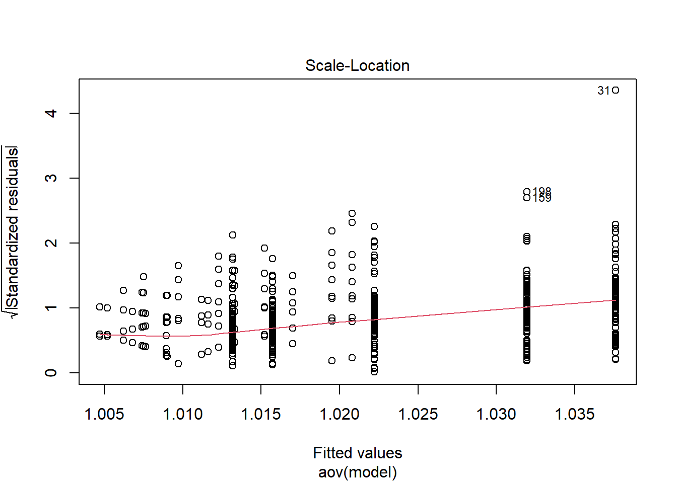
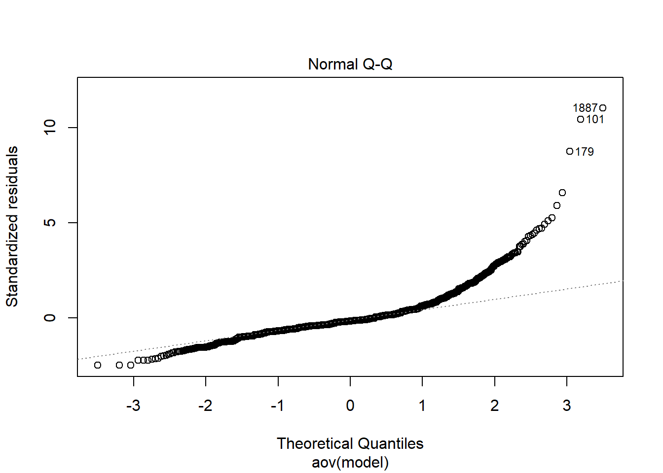
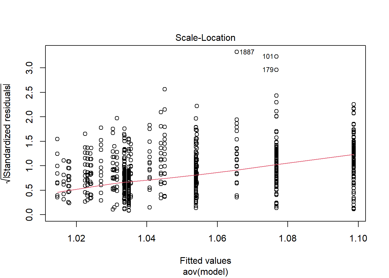
anova_assumptions_check(
  dat = conv_para_grp, outcome = 'Rhat_paragrp',
  factors = c('N_cat', 'N_items', 'N'),
  model = as.formula('Rhat_paragrp ~ N_cat*N_items*N'))


 ============================= 

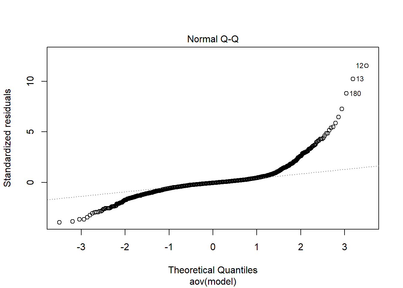
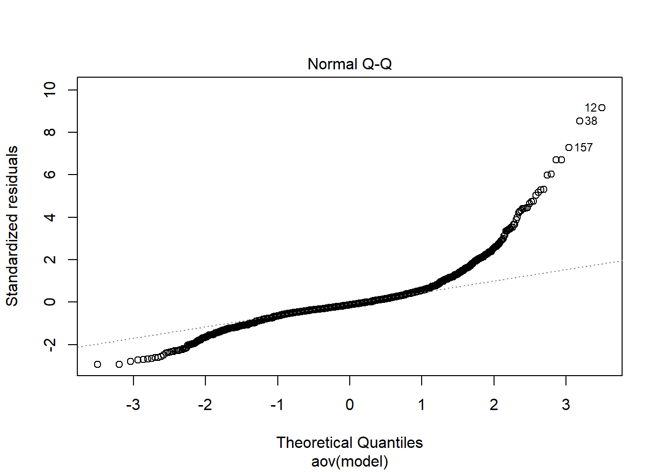
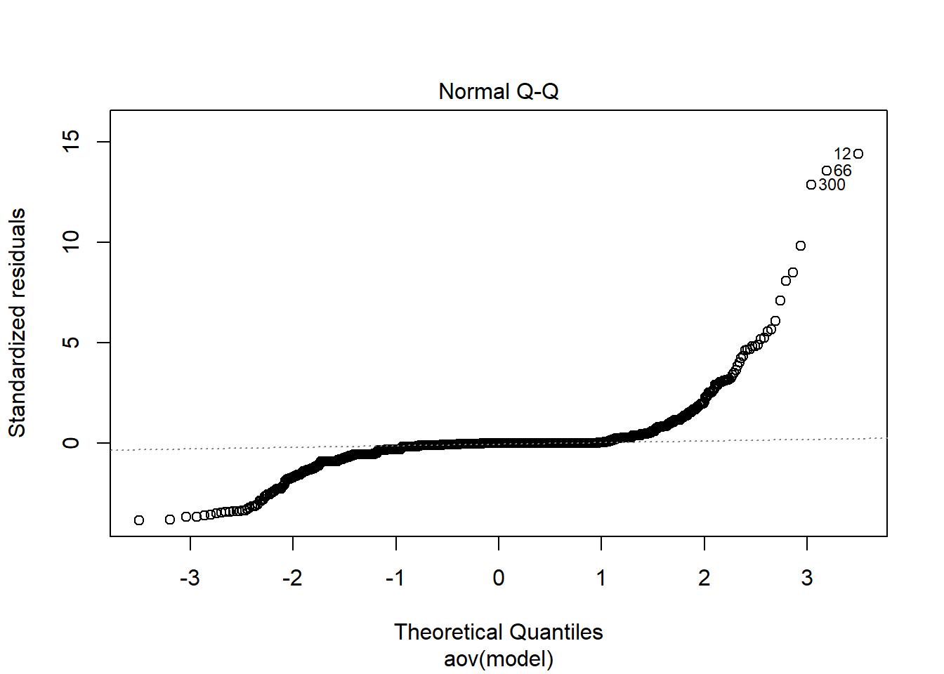
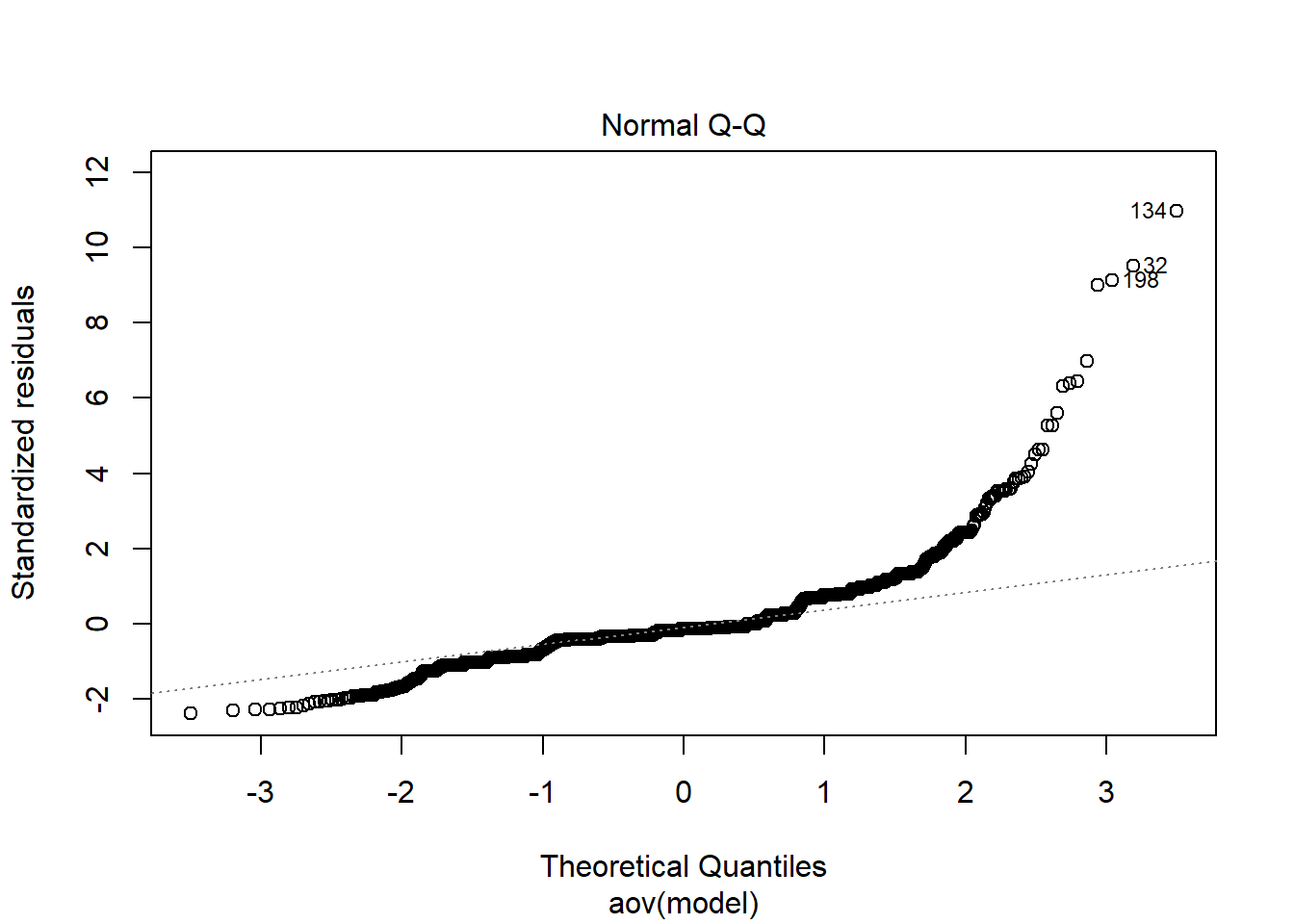
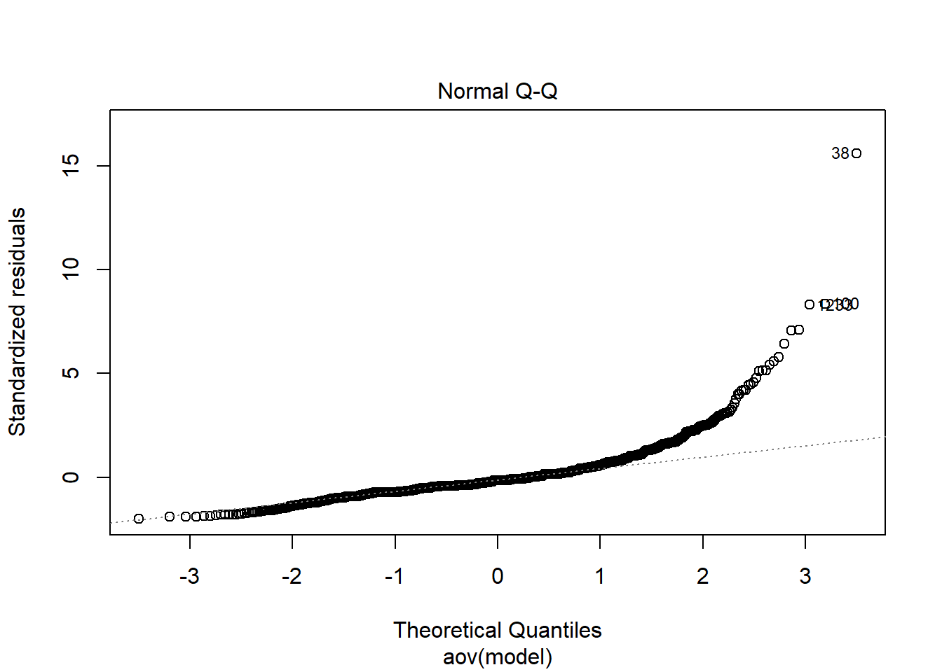
 Tests and Plots of Normality: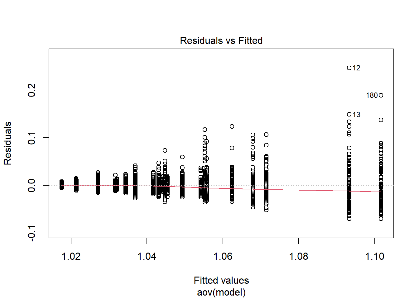


 Shapiro-Wilks Test of Normality of Residuals:

    Shapiro-Wilk normality test

data:  res
W = 0.8, p-value <0.0000000000000002


 K-S Test for Normality of Residuals:

Warning in ks.test(aov.out$residuals, "pnorm", alternative = "two.sided"): ties
should not be present for the Kolmogorov-Smirnov test


    One-sample Kolmogorov-Smirnov test

data:  aov.out$residuals
D = 0.5, p-value <0.0000000000000002
alternative hypothesis: two-sided

`stat_bin()` using `bins = 30`. Pick better value with `binwidth`.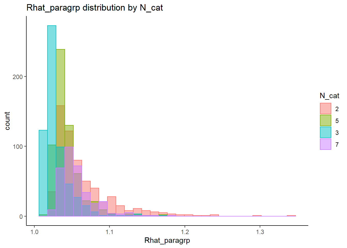

`stat_bin()` using `bins = 30`. Pick better value with `binwidth`.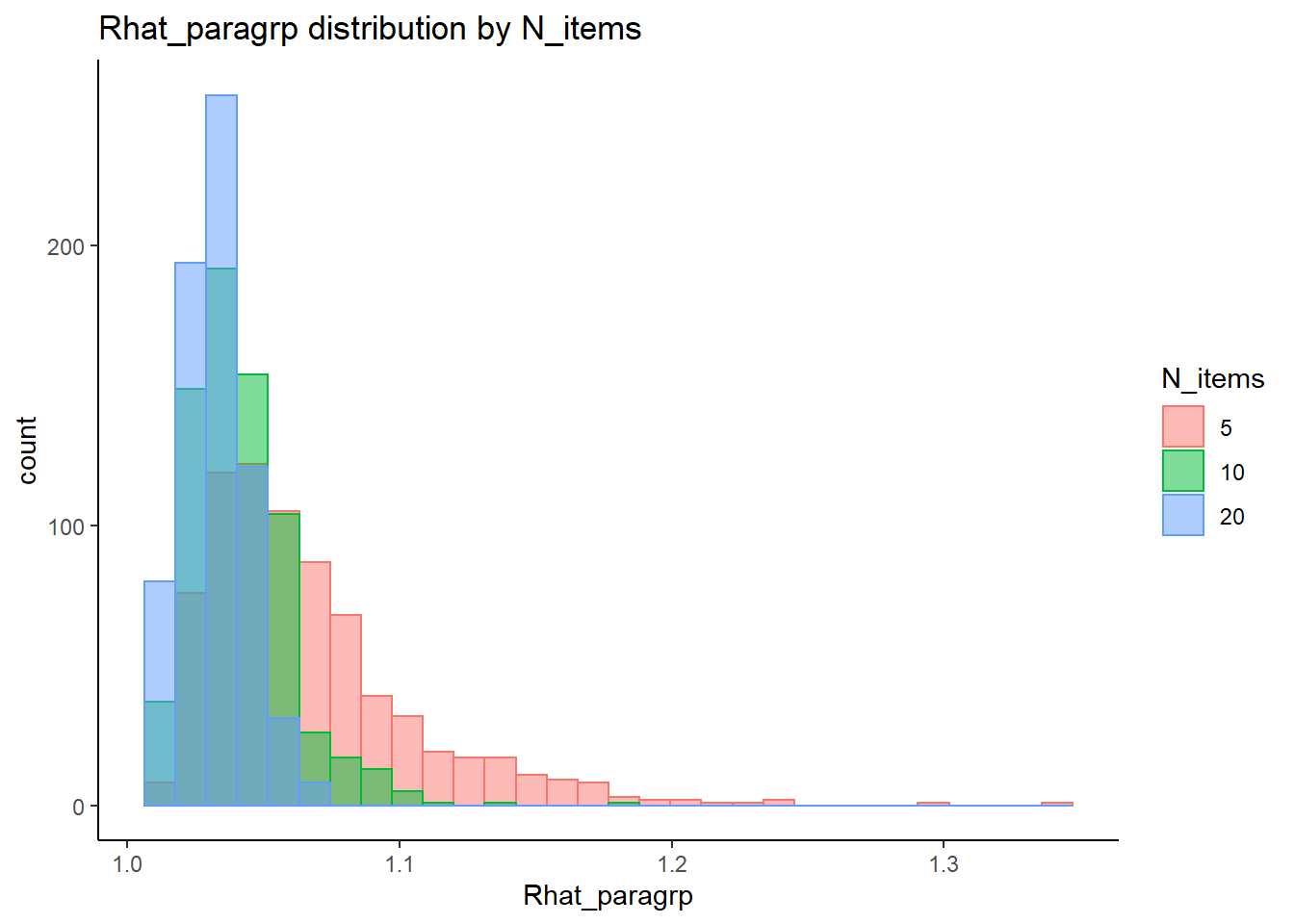

`stat_bin()` using `bins = 30`. Pick better value with `binwidth`.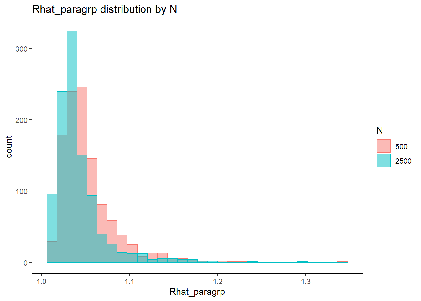


 ============================= 

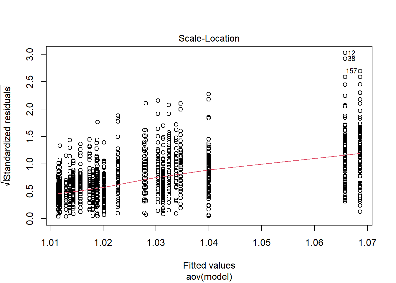
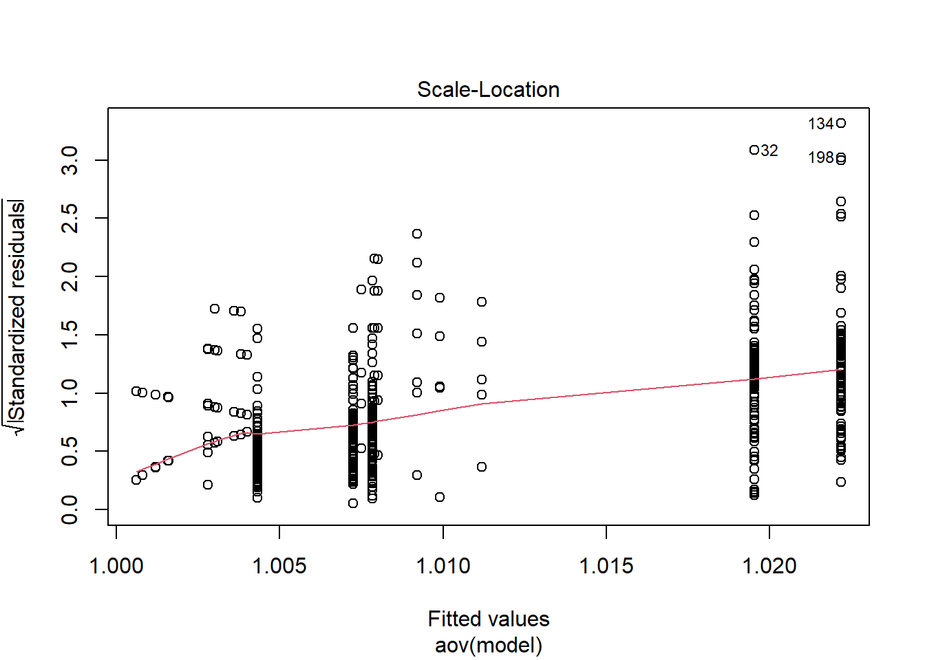
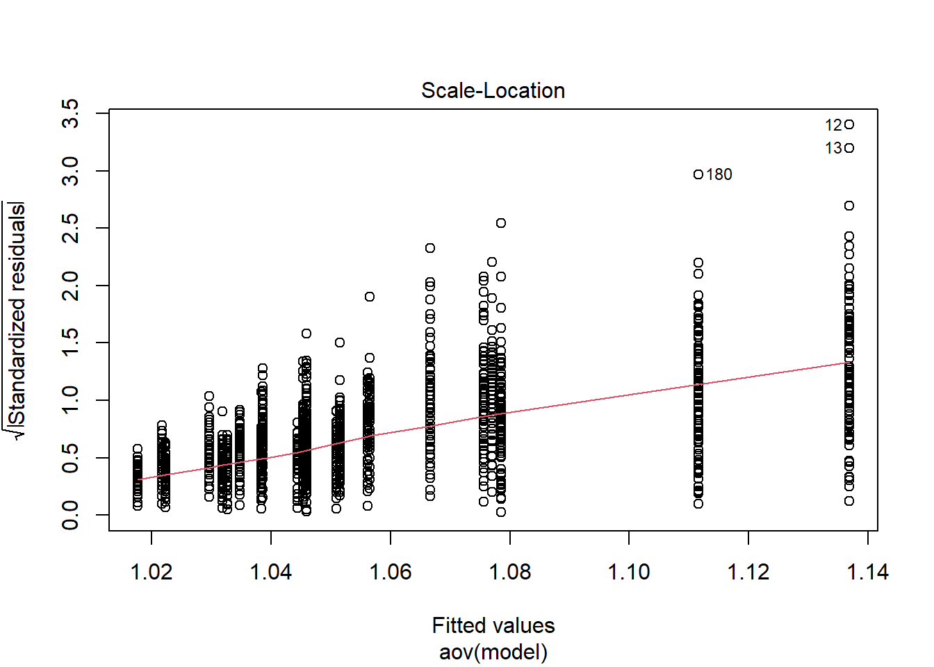
 Tests of Homogeneity of Variance

 
 Levenes Test:  N_cat 
 
 
Levene's Test for Homogeneity of Variance (center = "mean")
        Df F value              Pr(>F)    
group    3    79.9 <0.0000000000000002 ***
      2134                                
---
Signif. codes:  0 '***' 0.001 '**' 0.01 '*' 0.05 '.' 0.1 ' ' 1

 
 Levenes Test:  N_items 
 
 
Levene's Test for Homogeneity of Variance (center = "mean")
        Df F value              Pr(>F)    
group    2     241 <0.0000000000000002 ***
      2135                                
---
Signif. codes:  0 '***' 0.001 '**' 0.01 '*' 0.05 '.' 0.1 ' ' 1

 
 Levenes Test:  N 
 
 
Levene's Test for Homogeneity of Variance (center = "mean")
        Df F value Pr(>F)   
group    1    10.3 0.0014 **
      2136                  
---
Signif. codes:  0 '***' 0.001 '**' 0.01 '*' 0.05 '.' 0.1 ' ' 1

fit <- summary(aov(Rhat_paragrp ~ N_cat*N_items*N, data=conv_para_grp))
fit

                  Df Sum Sq Mean Sq F value               Pr(>F)    
N_cat              3  0.375  0.1249  269.23 < 0.0000000000000002 ***
N_items            2  0.440  0.2202  474.59 < 0.0000000000000002 ***
N                  1  0.042  0.0416   89.65 < 0.0000000000000002 ***
N_cat:N_items      6  0.107  0.0179   38.48 < 0.0000000000000002 ***
N_cat:N            3  0.005  0.0015    3.31                0.019 *  
N_items:N          2  0.003  0.0015    3.15                0.043 *  
N_cat:N_items:N    6  0.027  0.0045    9.75        0.00000000013 ***
Residuals       2114  0.981  0.0005                                 
---
Signif. codes:  0 '***' 0.001 '**' 0.01 '*' 0.05 '.' 0.1 ' ' 1

eta_est <- (fit[[1]]$`Sum Sq`/sum(fit[[1]]$`Sum Sq`))[1:7]
cbind(omega2(fit),p_omega2(fit), eta_est)

                omega^2 partial-omega^2 eta_est
N_cat            0.1886          0.2735 0.18933
N_items          0.2220          0.3070 0.22249
N                0.0208          0.0398 0.02101
N_cat:N_items    0.0527          0.0952 0.05412
N_cat:N          0.0016          0.0032 0.00232
N_items:N        0.0010          0.0020 0.00148
N_cat:N_items:N  0.0123          0.0240 0.01371

saved_omega[1,] <- omega2(fit)
saved_eta[1,] <- eta_est

Item Thresholds (\(\tau\))

conv_para_grp <- mydata %>%
  filter(parameter_group == "tau") %>%
  select(all_of(keep_cols)) %>%
  distinct()

## ANOVA on Rhat values
anova_assumptions_check(
  dat = conv_para_grp, outcome = 'Rhat_paragrp',
  factors = c('N_cat', 'N_items', 'N'),
  model = as.formula('Rhat_paragrp ~ N_cat*N_items*N'))


 ============================= 

 Tests and Plots of Normality: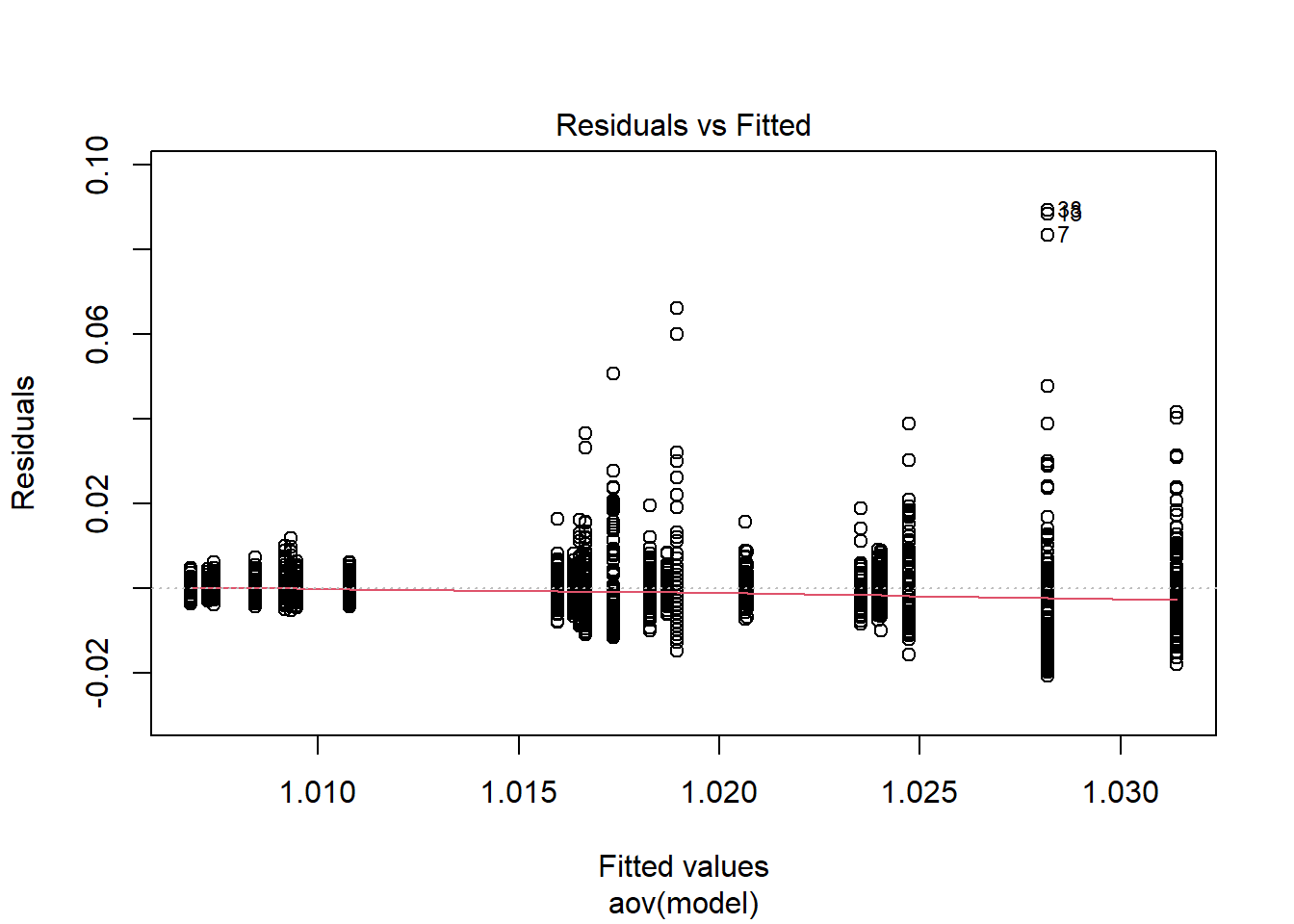


 Shapiro-Wilks Test of Normality of Residuals:

    Shapiro-Wilk normality test

data:  res
W = 0.7, p-value <0.0000000000000002


 K-S Test for Normality of Residuals:

Warning in ks.test(aov.out$residuals, "pnorm", alternative = "two.sided"): ties
should not be present for the Kolmogorov-Smirnov test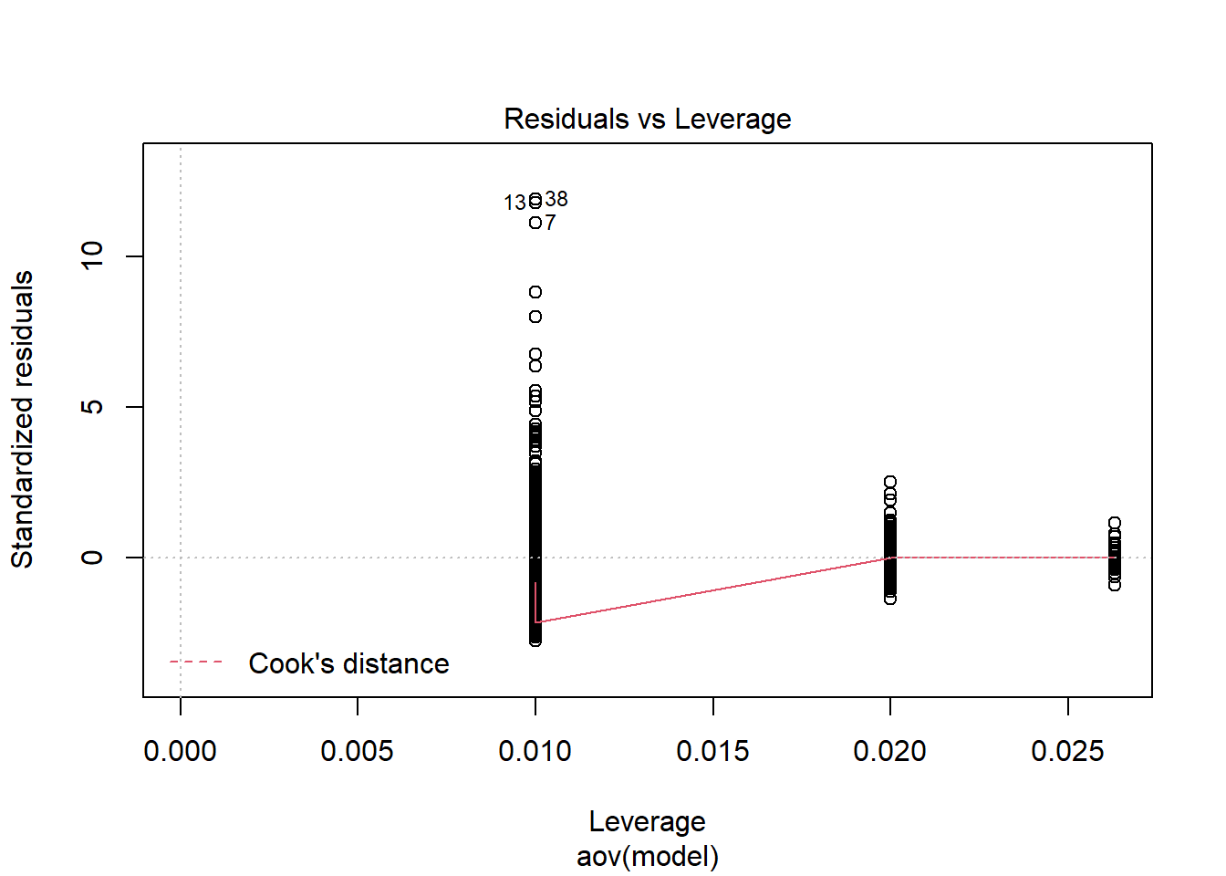


    One-sample Kolmogorov-Smirnov test

data:  aov.out$residuals
D = 0.5, p-value <0.0000000000000002
alternative hypothesis: two-sided

`stat_bin()` using `bins = 30`. Pick better value with `binwidth`.

`stat_bin()` using `bins = 30`. Pick better value with `binwidth`.

`stat_bin()` using `bins = 30`. Pick better value with `binwidth`.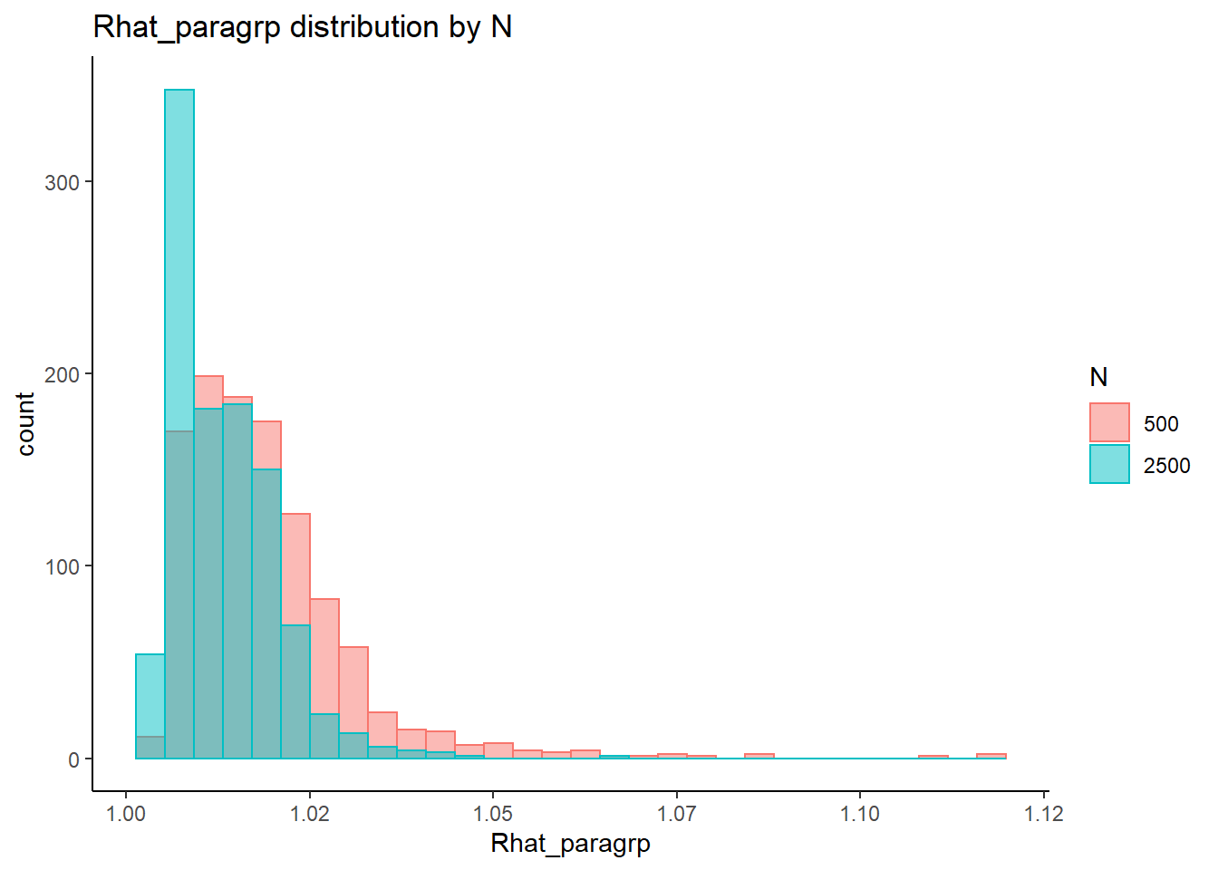


 ============================= 

 Tests of Homogeneity of Variance

 
 Levenes Test:  N_cat 
 
 
Levene's Test for Homogeneity of Variance (center = "mean")
        Df F value              Pr(>F)    
group    3    32.3 <0.0000000000000002 ***
      2134                                
---
Signif. codes:  0 '***' 0.001 '**' 0.01 '*' 0.05 '.' 0.1 ' ' 1

 
 Levenes Test:  N_items 
 
 
Levene's Test for Homogeneity of Variance (center = "mean")
        Df F value              Pr(>F)    
group    2    93.2 <0.0000000000000002 ***
      2135                                
---
Signif. codes:  0 '***' 0.001 '**' 0.01 '*' 0.05 '.' 0.1 ' ' 1

 
 Levenes Test:  N 
 
 
Levene's Test for Homogeneity of Variance (center = "mean")
        Df F value              Pr(>F)    
group    1      76 <0.0000000000000002 ***
      2136                                
---
Signif. codes:  0 '***' 0.001 '**' 0.01 '*' 0.05 '.' 0.1 ' ' 1

fit <- summary(aov(Rhat_paragrp ~ N_cat*N_items*N, data=conv_para_grp))
fit

                  Df Sum Sq Mean Sq F value              Pr(>F)    
N_cat              3 0.0547 0.01824  319.94 <0.0000000000000002 ***
N_items            2 0.0237 0.01183  207.48 <0.0000000000000002 ***
N                  1 0.0146 0.01459  255.89 <0.0000000000000002 ***
N_cat:N_items      6 0.0062 0.00103   18.05 <0.0000000000000002 ***
N_cat:N            3 0.0008 0.00026    4.62              0.0032 ** 
N_items:N          2 0.0047 0.00233   40.90 <0.0000000000000002 ***
N_cat:N_items:N    6 0.0004 0.00006    1.10              0.3580    
Residuals       2114 0.1205 0.00006                                
---
Signif. codes:  0 '***' 0.001 '**' 0.01 '*' 0.05 '.' 0.1 ' ' 1

eta_est <- (fit[[1]]$`Sum Sq`/sum(fit[[1]]$`Sum Sq`))[1:7]
cbind(omega2(fit),p_omega2(fit), eta_est)

                omega^2 partial-omega^2 eta_est
N_cat            0.2419          0.3092 0.24267
N_items          0.1044          0.1619 0.10492
N                0.0644          0.1065 0.06470
N_cat:N_items    0.0259          0.0457 0.02738
N_cat:N          0.0027          0.0050 0.00350
N_items:N        0.0202          0.0360 0.02068
N_cat:N_items:N  0.0002          0.0003 0.00167

saved_omega[2,] <- omega2(fit)
saved_eta[2,] <- eta_est

Latent Response Variance (\(\theta\))

conv_para_grp <- mydata %>%
  filter(parameter_group == "theta") %>%
  select(all_of(keep_cols)) %>%
  distinct()

## ANOVA on Rhat values
anova_assumptions_check(
  dat = conv_para_grp, outcome = 'Rhat_paragrp',
  factors = c('N_cat', 'N_items', 'N'),
  model = as.formula('Rhat_paragrp ~ N_cat*N_items*N'))


 ============================= 

 Tests and Plots of Normality: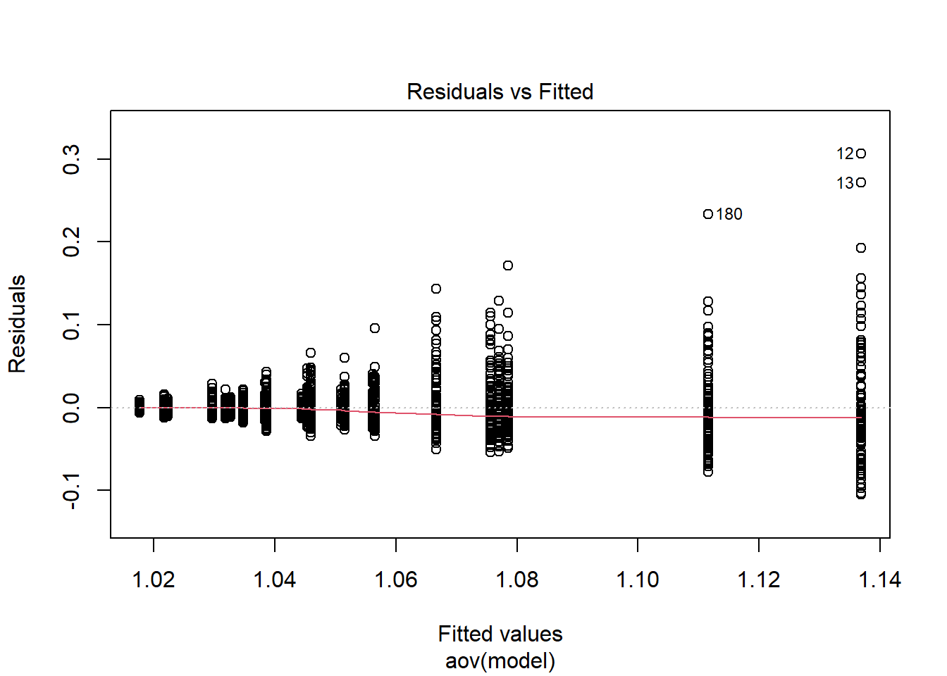


 Shapiro-Wilks Test of Normality of Residuals:

    Shapiro-Wilk normality test

data:  res
W = 0.8, p-value <0.0000000000000002


 K-S Test for Normality of Residuals:

Warning in ks.test(aov.out$residuals, "pnorm", alternative = "two.sided"): ties
should not be present for the Kolmogorov-Smirnov test


    One-sample Kolmogorov-Smirnov test

data:  aov.out$residuals
D = 0.5, p-value <0.0000000000000002
alternative hypothesis: two-sided

`stat_bin()` using `bins = 30`. Pick better value with `binwidth`.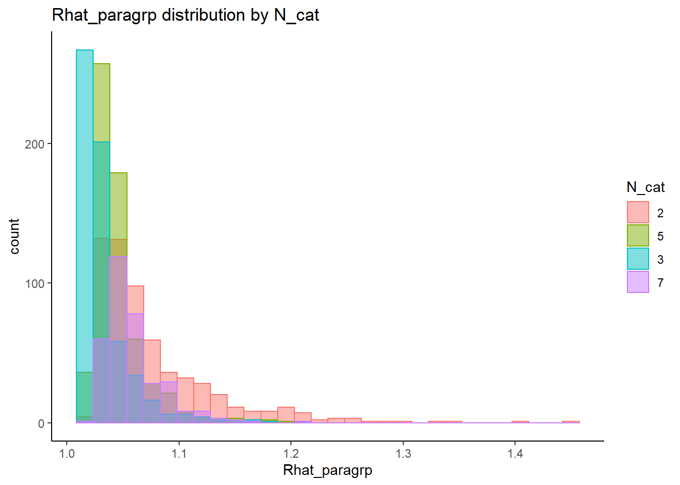

`stat_bin()` using `bins = 30`. Pick better value with `binwidth`.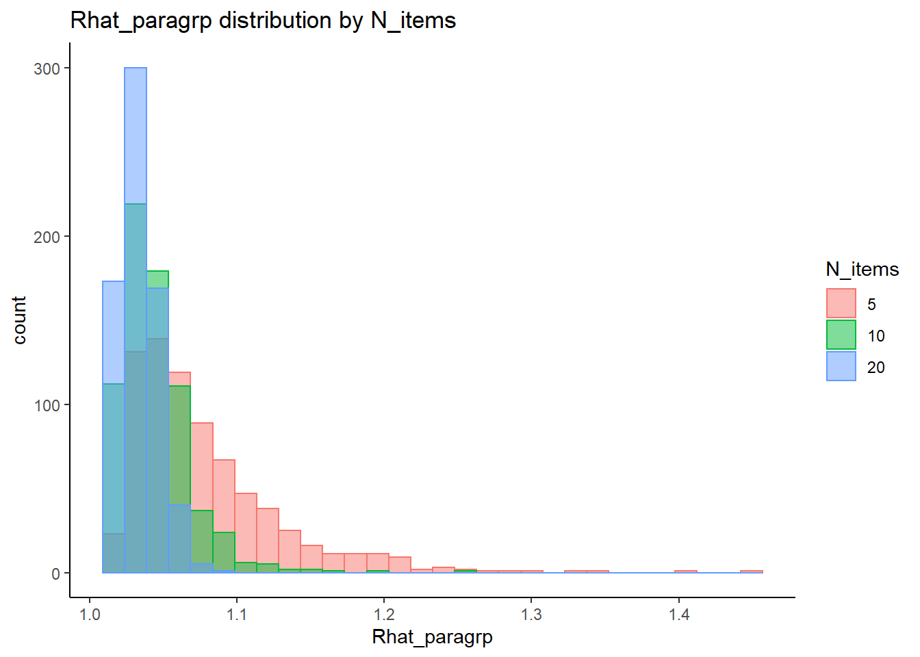

`stat_bin()` using `bins = 30`. Pick better value with `binwidth`.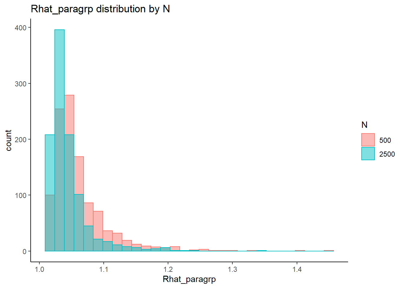


 ============================= 

 Tests of Homogeneity of Variance

 
 Levenes Test:  N_cat 
 
 
Levene's Test for Homogeneity of Variance (center = "mean")
        Df F value              Pr(>F)    
group    3     124 <0.0000000000000002 ***
      2134                                
---
Signif. codes:  0 '***' 0.001 '**' 0.01 '*' 0.05 '.' 0.1 ' ' 1

 
 Levenes Test:  N_items 
 
 
Levene's Test for Homogeneity of Variance (center = "mean")
        Df F value              Pr(>F)    
group    2     258 <0.0000000000000002 ***
      2135                                
---
Signif. codes:  0 '***' 0.001 '**' 0.01 '*' 0.05 '.' 0.1 ' ' 1

 
 Levenes Test:  N 
 
 
Levene's Test for Homogeneity of Variance (center = "mean")
        Df F value           Pr(>F)    
group    1    54.8 0.00000000000019 ***
      2136                             
---
Signif. codes:  0 '***' 0.001 '**' 0.01 '*' 0.05 '.' 0.1 ' ' 1

fit <- summary(aov(Rhat_paragrp ~ N_cat*N_items*N, data=conv_para_grp))
fit

                  Df Sum Sq Mean Sq F value               Pr(>F)    
N_cat              3  0.614   0.205  288.25 < 0.0000000000000002 ***
N_items            2  0.741   0.371  522.07 < 0.0000000000000002 ***
N                  1  0.138   0.138  194.78 < 0.0000000000000002 ***
N_cat:N_items      6  0.254   0.042   59.55 < 0.0000000000000002 ***
N_cat:N            3  0.006   0.002    2.96                0.031 *  
N_items:N          2  0.032   0.016   22.37        0.00000000024 ***
N_cat:N_items:N    6  0.008   0.001    1.88                0.080 .  
Residuals       2114  1.501   0.001                                 
---
Signif. codes:  0 '***' 0.001 '**' 0.01 '*' 0.05 '.' 0.1 ' ' 1

eta_est <- (fit[[1]]$`Sum Sq`/sum(fit[[1]]$`Sum Sq`))[1:7]
cbind(omega2(fit),p_omega2(fit), eta_est)

                omega^2 partial-omega^2 eta_est
N_cat            0.1857          0.2873 0.18637
N_items          0.2246          0.3277 0.22504
N                0.0418          0.0831 0.04198
N_cat:N_items    0.0757          0.1411 0.07700
N_cat:N          0.0013          0.0027 0.00192
N_items:N        0.0092          0.0196 0.00964
N_cat:N_items:N  0.0011          0.0025 0.00243

saved_omega[3,] <- omega2(fit)
saved_eta[3,] <- eta_est

Response Time Intercepts (\(\beta_{lrt}\))

conv_para_grp <- mydata %>%
  filter(parameter_group == "beta_lrt") %>%
  select(all_of(keep_cols)) %>%
  distinct()

## ANOVA on Rhat values
anova_assumptions_check(
  dat = conv_para_grp, outcome = 'Rhat_paragrp',
  factors = c('N_cat', 'N_items', 'N'),
  model = as.formula('Rhat_paragrp ~ N_cat*N_items*N'))


 ============================= 

 Tests and Plots of Normality: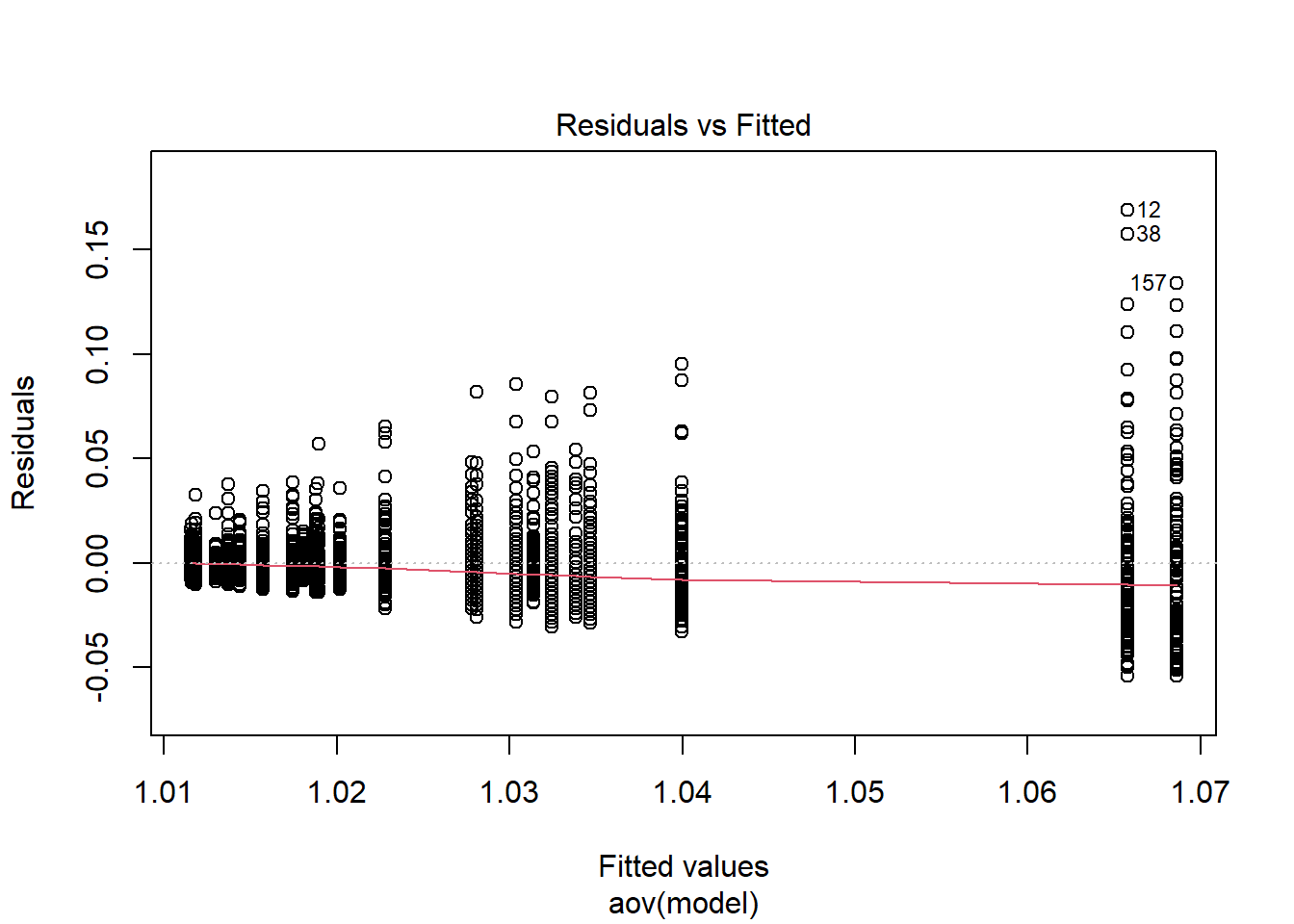


 Shapiro-Wilks Test of Normality of Residuals:

    Shapiro-Wilk normality test

data:  res
W = 0.8, p-value <0.0000000000000002


 K-S Test for Normality of Residuals:

Warning in ks.test(aov.out$residuals, "pnorm", alternative = "two.sided"): ties
should not be present for the Kolmogorov-Smirnov test


    One-sample Kolmogorov-Smirnov test

data:  aov.out$residuals
D = 0.5, p-value <0.0000000000000002
alternative hypothesis: two-sided

`stat_bin()` using `bins = 30`. Pick better value with `binwidth`.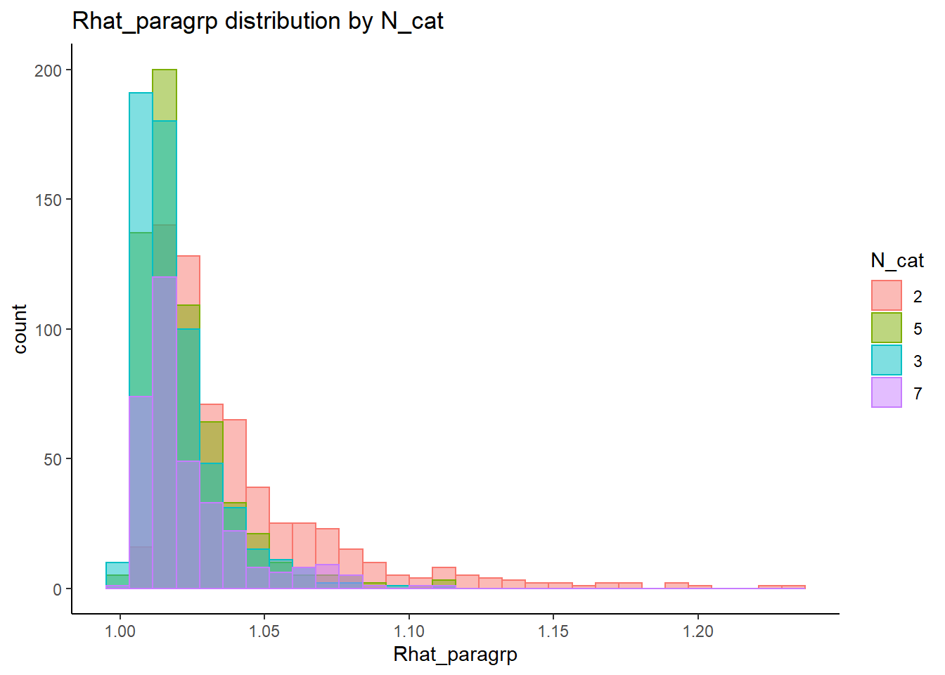

`stat_bin()` using `bins = 30`. Pick better value with `binwidth`.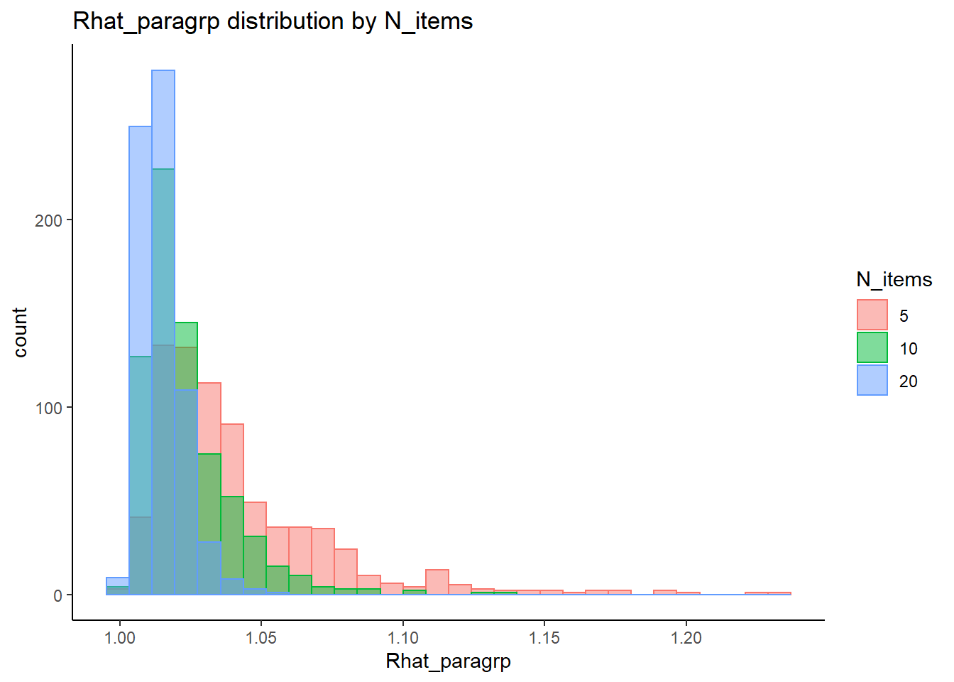

`stat_bin()` using `bins = 30`. Pick better value with `binwidth`.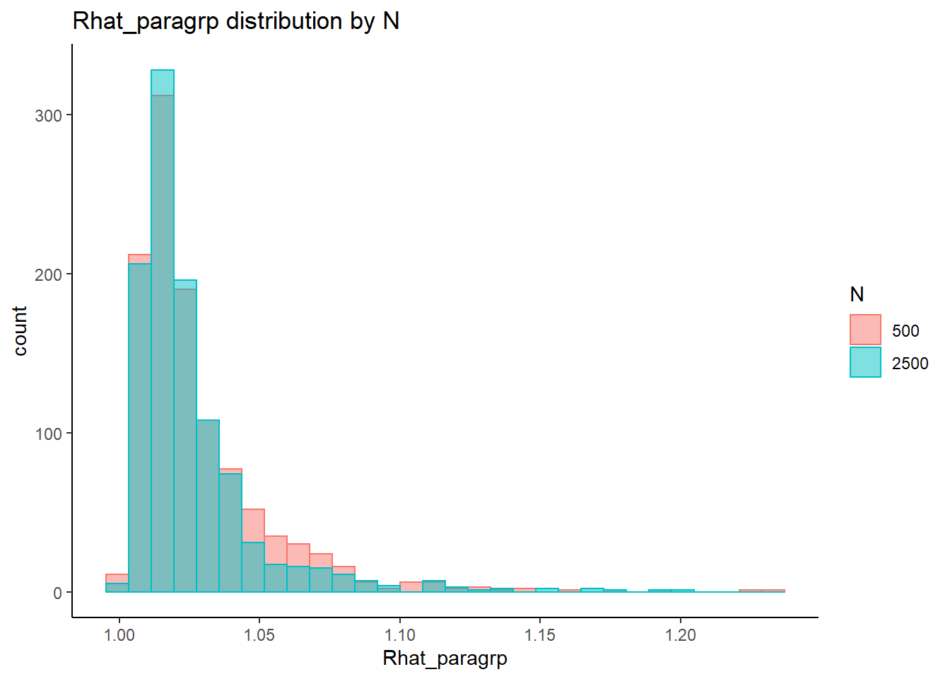


 ============================= 

 Tests of Homogeneity of Variance

 
 Levenes Test:  N_cat 
 
 
Levene's Test for Homogeneity of Variance (center = "mean")
        Df F value              Pr(>F)    
group    3    86.4 <0.0000000000000002 ***
      2134                                
---
Signif. codes:  0 '***' 0.001 '**' 0.01 '*' 0.05 '.' 0.1 ' ' 1

 
 Levenes Test:  N_items 
 
 
Levene's Test for Homogeneity of Variance (center = "mean")
        Df F value              Pr(>F)    
group    2     233 <0.0000000000000002 ***
      2135                                
---
Signif. codes:  0 '***' 0.001 '**' 0.01 '*' 0.05 '.' 0.1 ' ' 1

 
 Levenes Test:  N 
 
 
Levene's Test for Homogeneity of Variance (center = "mean")
        Df F value Pr(>F)   
group    1    8.15 0.0043 **
      2136                  
---
Signif. codes:  0 '***' 0.001 '**' 0.01 '*' 0.05 '.' 0.1 ' ' 1

fit <- summary(aov(Rhat_paragrp ~ N_cat*N_items*N, data=conv_para_grp))
fit

                  Df Sum Sq Mean Sq F value              Pr(>F)    
N_cat              3  0.168  0.0560  163.03 <0.0000000000000002 ***
N_items            2  0.261  0.1303  379.56 <0.0000000000000002 ***
N                  1  0.002  0.0018    5.35               0.021 *  
N_cat:N_items      6  0.068  0.0113   32.80 <0.0000000000000002 ***
N_cat:N            3  0.001  0.0004    1.04               0.375    
N_items:N          2  0.001  0.0007    1.94               0.145    
N_cat:N_items:N    6  0.003  0.0006    1.69               0.118    
Residuals       2114  0.726  0.0003                                
---
Signif. codes:  0 '***' 0.001 '**' 0.01 '*' 0.05 '.' 0.1 ' ' 1

eta_est <- (fit[[1]]$`Sum Sq`/sum(fit[[1]]$`Sum Sq`))[1:7]
cbind(omega2(fit),p_omega2(fit), eta_est)

                omega^2 partial-omega^2  eta_est
N_cat            0.1357          0.1852 0.136558
N_items          0.2113          0.2615 0.211958
N                0.0012          0.0020 0.001493
N_cat:N_items    0.0533          0.0819 0.054942
N_cat:N          0.0000          0.0001 0.000868
N_items:N        0.0005          0.0009 0.001081
N_cat:N_items:N  0.0012          0.0019 0.002839

saved_omega[4,] <- omega2(fit)
saved_eta[4,] <- eta_est

Response Time Precision (\(\sigma_{lrt}\))

conv_para_grp <- mydata %>%
  filter(parameter_group == "sigma_lrt") %>%
  select(all_of(keep_cols)) %>%
  distinct()

## ANOVA on Rhat values
anova_assumptions_check(
  dat = conv_para_grp, outcome = 'Rhat_paragrp',
  factors = c('N_cat', 'N_items', 'N'),
  model = as.formula('Rhat_paragrp ~ N_cat*N_items*N'))


 ============================= 

 Tests and Plots of Normality: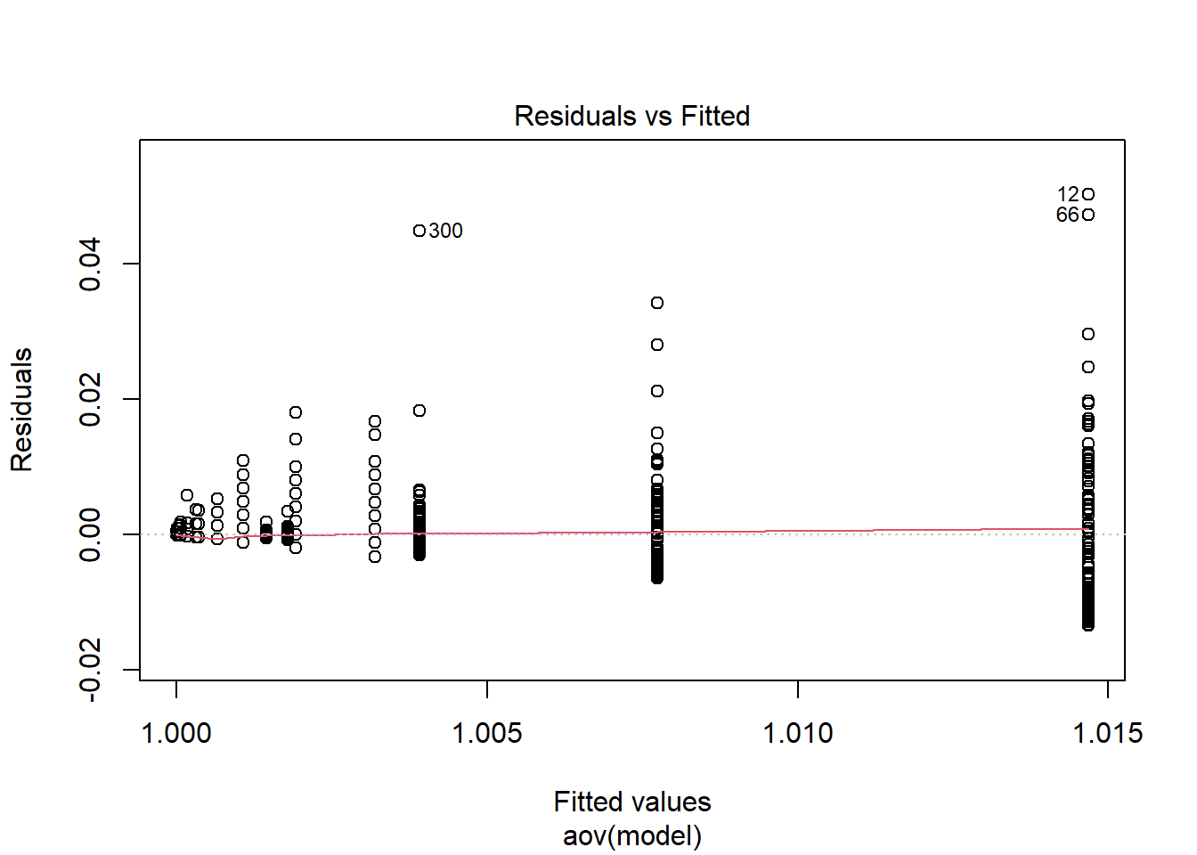


 Shapiro-Wilks Test of Normality of Residuals:

    Shapiro-Wilk normality test

data:  res
W = 0.5, p-value <0.0000000000000002


 K-S Test for Normality of Residuals:

Warning in ks.test(aov.out$residuals, "pnorm", alternative = "two.sided"): ties
should not be present for the Kolmogorov-Smirnov test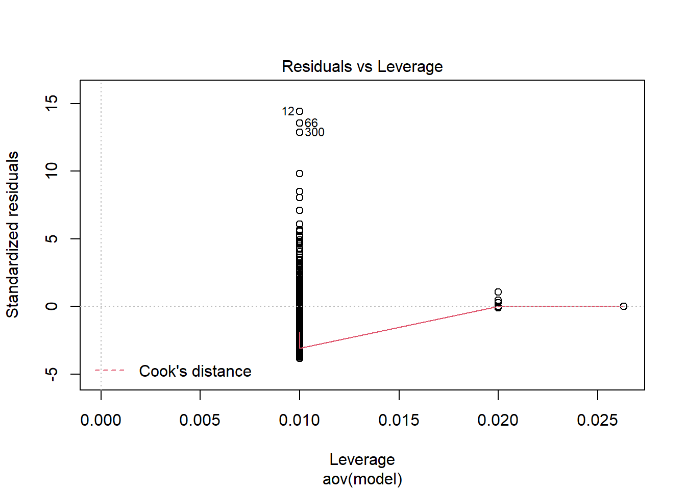


    One-sample Kolmogorov-Smirnov test

data:  aov.out$residuals
D = 0.5, p-value <0.0000000000000002
alternative hypothesis: two-sided

`stat_bin()` using `bins = 30`. Pick better value with `binwidth`.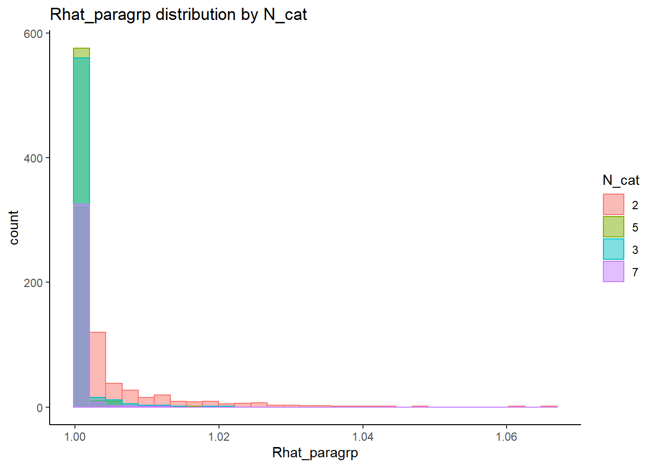

`stat_bin()` using `bins = 30`. Pick better value with `binwidth`.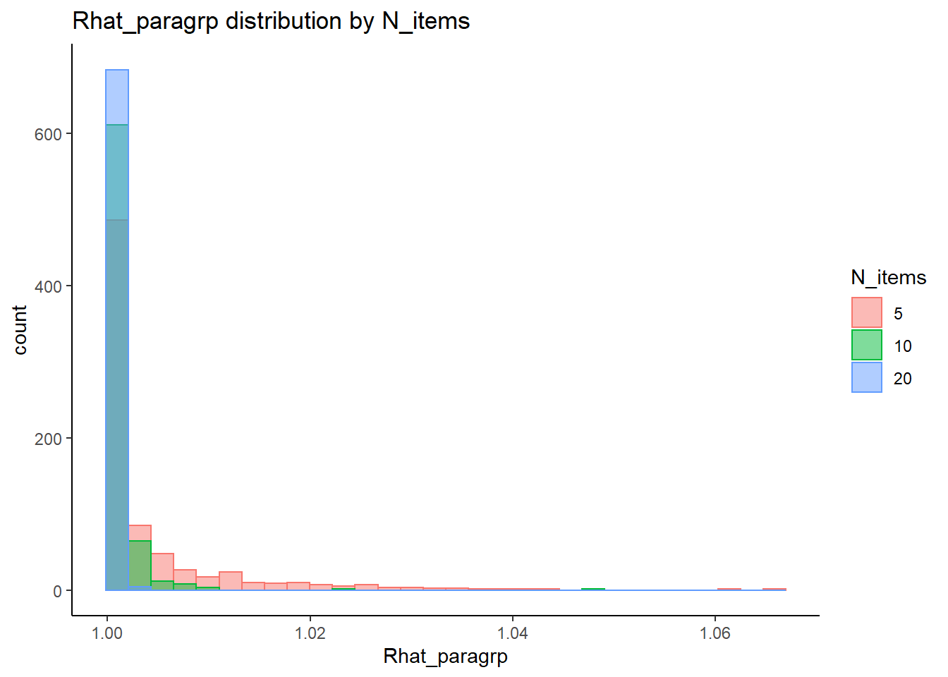

`stat_bin()` using `bins = 30`. Pick better value with `binwidth`.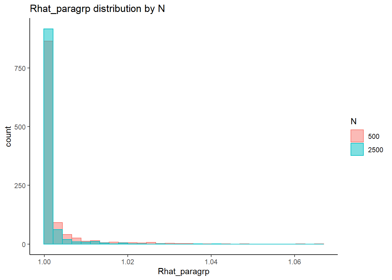


 ============================= 

 Tests of Homogeneity of Variance

 
 Levenes Test:  N_cat 
 
 
Levene's Test for Homogeneity of Variance (center = "mean")
        Df F value              Pr(>F)    
group    3     202 <0.0000000000000002 ***
      2134                                
---
Signif. codes:  0 '***' 0.001 '**' 0.01 '*' 0.05 '.' 0.1 ' ' 1

 
 Levenes Test:  N_items 
 
 
Levene's Test for Homogeneity of Variance (center = "mean")
        Df F value              Pr(>F)    
group    2     285 <0.0000000000000002 ***
      2135                                
---
Signif. codes:  0 '***' 0.001 '**' 0.01 '*' 0.05 '.' 0.1 ' ' 1

 
 Levenes Test:  N 
 
 
Levene's Test for Homogeneity of Variance (center = "mean")
        Df F value              Pr(>F)    
group    1      80 <0.0000000000000002 ***
      2136                                
---
Signif. codes:  0 '***' 0.001 '**' 0.01 '*' 0.05 '.' 0.1 ' ' 1

fit <- summary(aov(Rhat_paragrp ~ N_cat*N_items*N, data=conv_para_grp))
fit

                  Df  Sum Sq  Mean Sq F value               Pr(>F)    
N_cat              3 0.00853 0.002843  231.39 < 0.0000000000000002 ***
N_items            2 0.00628 0.003140  255.63 < 0.0000000000000002 ***
N                  1 0.00103 0.001026   83.53 < 0.0000000000000002 ***
N_cat:N_items      6 0.00674 0.001123   91.39 < 0.0000000000000002 ***
N_cat:N            3 0.00089 0.000296   24.07   0.0000000000000026 ***
N_items:N          2 0.00086 0.000431   35.04   0.0000000000000011 ***
N_cat:N_items:N    6 0.00034 0.000056    4.55              0.00014 ***
Residuals       2114 0.02597 0.000012                                 
---
Signif. codes:  0 '***' 0.001 '**' 0.01 '*' 0.05 '.' 0.1 ' ' 1

eta_est <- (fit[[1]]$`Sum Sq`/sum(fit[[1]]$`Sum Sq`))[1:7]
cbind(omega2(fit),p_omega2(fit), eta_est)

                omega^2 partial-omega^2 eta_est
N_cat            0.1677          0.2443 0.16845
N_items          0.1235          0.1924 0.12406
N                0.0200          0.0372 0.02027
N_cat:N_items    0.1316          0.2023 0.13306
N_cat:N          0.0168          0.0314 0.01752
N_items:N        0.0165          0.0309 0.01701
N_cat:N_items:N  0.0052          0.0099 0.00662

saved_omega[5,] <- omega2(fit)
saved_eta[5,] <- eta_est

Response Time Factor Precision (\(\sigma_s\))

conv_para_grp <- mydata %>%
  filter(parameter_group == "sigma_s") %>%
  select(all_of(keep_cols)) %>%
  distinct()

## ANOVA on Rhat values
anova_assumptions_check(
  dat = conv_para_grp, outcome = 'Rhat_paragrp',
  factors = c('N_cat', 'N_items', 'N'),
  model = as.formula('Rhat_paragrp ~ N_cat*N_items*N'))


 ============================= 

 Tests and Plots of Normality: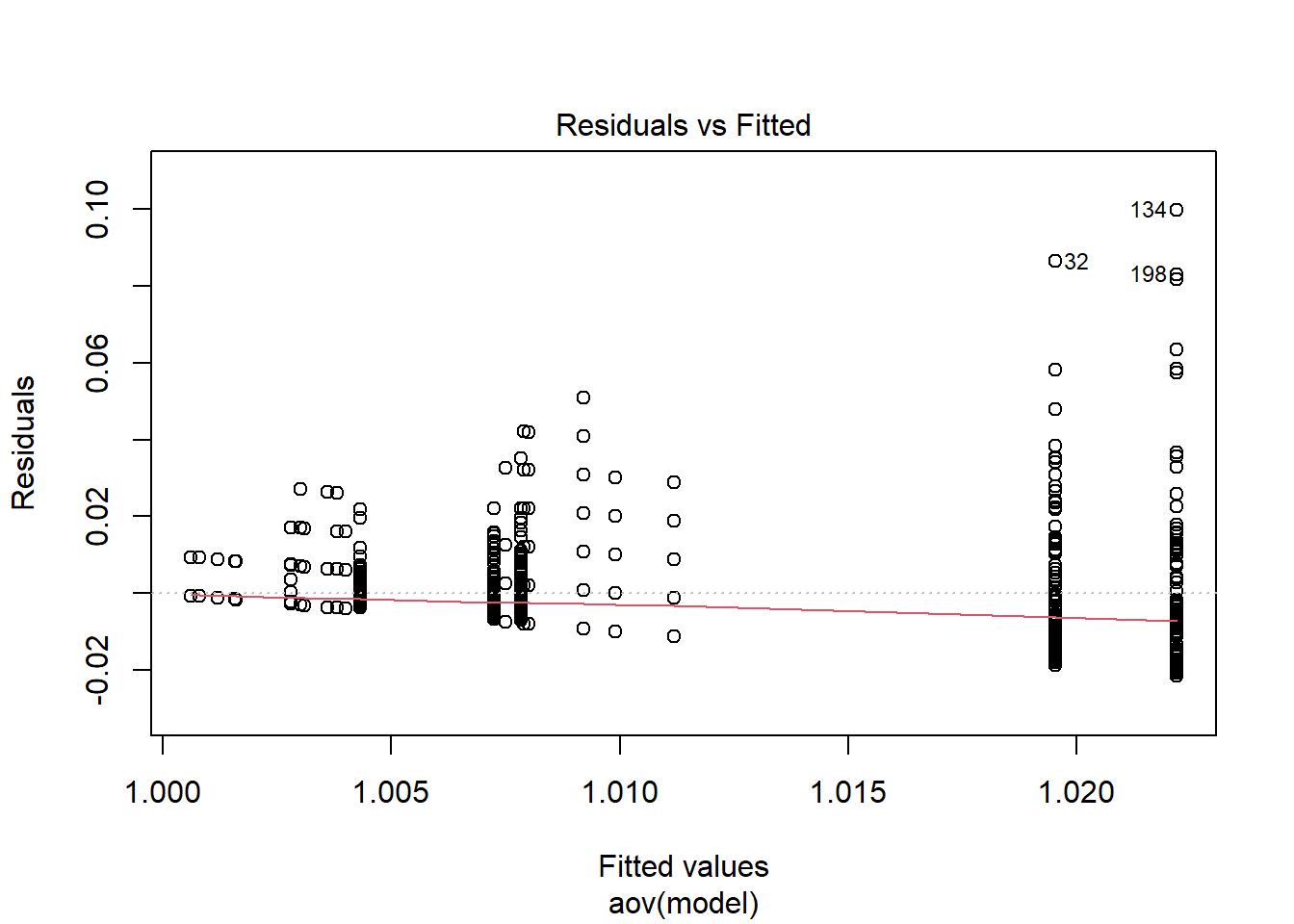


 Shapiro-Wilks Test of Normality of Residuals:

    Shapiro-Wilk normality test

data:  res
W = 0.8, p-value <0.0000000000000002


 K-S Test for Normality of Residuals:

Warning in ks.test(aov.out$residuals, "pnorm", alternative = "two.sided"): ties
should not be present for the Kolmogorov-Smirnov test


    One-sample Kolmogorov-Smirnov test

data:  aov.out$residuals
D = 0.5, p-value <0.0000000000000002
alternative hypothesis: two-sided

`stat_bin()` using `bins = 30`. Pick better value with `binwidth`.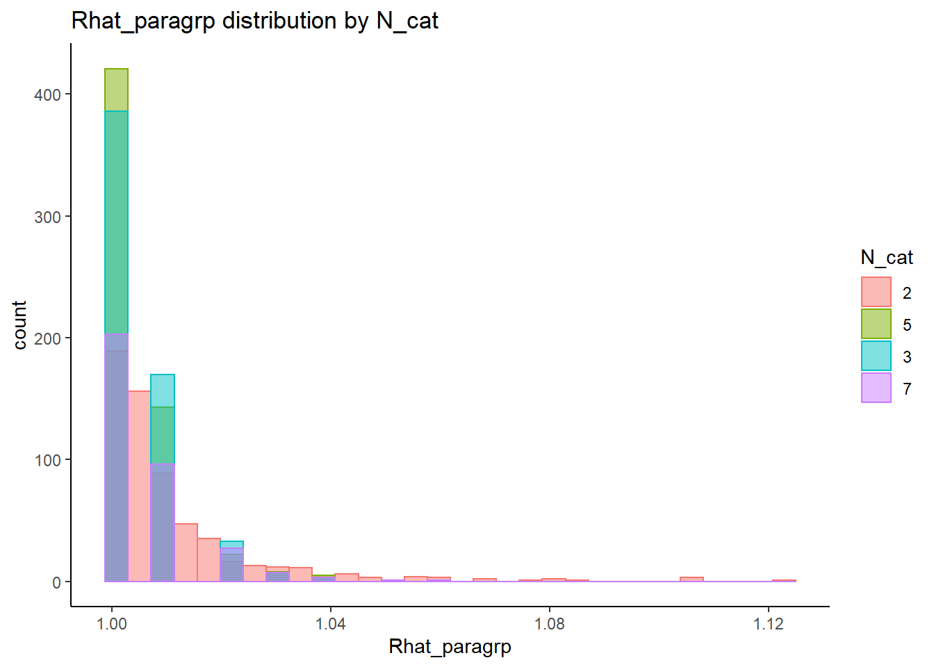

`stat_bin()` using `bins = 30`. Pick better value with `binwidth`.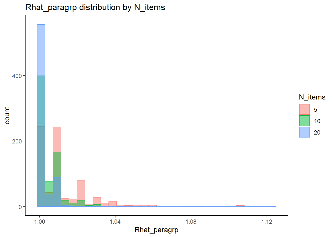

`stat_bin()` using `bins = 30`. Pick better value with `binwidth`.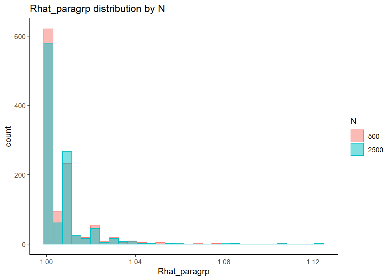


 ============================= 

 Tests of Homogeneity of Variance

 
 Levenes Test:  N_cat 
 
 
Levene's Test for Homogeneity of Variance (center = "mean")
        Df F value              Pr(>F)    
group    3    34.7 <0.0000000000000002 ***
      2134                                
---
Signif. codes:  0 '***' 0.001 '**' 0.01 '*' 0.05 '.' 0.1 ' ' 1

 
 Levenes Test:  N_items 
 
 
Levene's Test for Homogeneity of Variance (center = "mean")
        Df F value              Pr(>F)    
group    2     190 <0.0000000000000002 ***
      2135                                
---
Signif. codes:  0 '***' 0.001 '**' 0.01 '*' 0.05 '.' 0.1 ' ' 1

 
 Levenes Test:  N 
 
 
Levene's Test for Homogeneity of Variance (center = "mean")
        Df F value Pr(>F)
group    1    0.03   0.86
      2136

fit <- summary(aov(Rhat_paragrp ~ N_cat*N_items*N, data=conv_para_grp))
fit

                  Df Sum Sq Mean Sq F value              Pr(>F)    
N_cat              3 0.0167 0.00555   66.57 <0.0000000000000002 ***
N_items            2 0.0408 0.02039  244.42 <0.0000000000000002 ***
N                  1 0.0000 0.00003    0.31                0.58    
N_cat:N_items      6 0.0080 0.00134   16.03 <0.0000000000000002 ***
N_cat:N            3 0.0001 0.00004    0.44                0.73    
N_items:N          2 0.0005 0.00023    2.82                0.06 .  
N_cat:N_items:N    6 0.0003 0.00005    0.60                0.73    
Residuals       2114 0.1763 0.00008                                
---
Signif. codes:  0 '***' 0.001 '**' 0.01 '*' 0.05 '.' 0.1 ' ' 1

eta_est <- (fit[[1]]$`Sum Sq`/sum(fit[[1]]$`Sum Sq`))[1:7]
cbind(omega2(fit),p_omega2(fit), eta_est)

                omega^2 partial-omega^2  eta_est
N_cat            0.0676          0.0843 0.068641
N_items          0.1673          0.1855 0.168011
N               -0.0002         -0.0003 0.000106
N_cat:N_items    0.0310          0.0405 0.033056
N_cat:N         -0.0006         -0.0008 0.000452
N_items:N        0.0012          0.0017 0.001935
N_cat:N_items:N -0.0008         -0.0011 0.001236

saved_omega[6,] <- omega2(fit)
saved_eta[6,] <- eta_est

Factor Covariance (\(\sigma_{st}\))

conv_para_grp <- mydata %>%
  filter(parameter_group == "sigma_st") %>%
  select(all_of(keep_cols)) %>%
  distinct()

## ANOVA on Rhat values
anova_assumptions_check(
  dat = conv_para_grp, outcome = 'Rhat_paragrp',
  factors = c('N_cat', 'N_items', 'N'),
  model = as.formula('Rhat_paragrp ~ N_cat*N_items*N'))


 ============================= 

 Tests and Plots of Normality: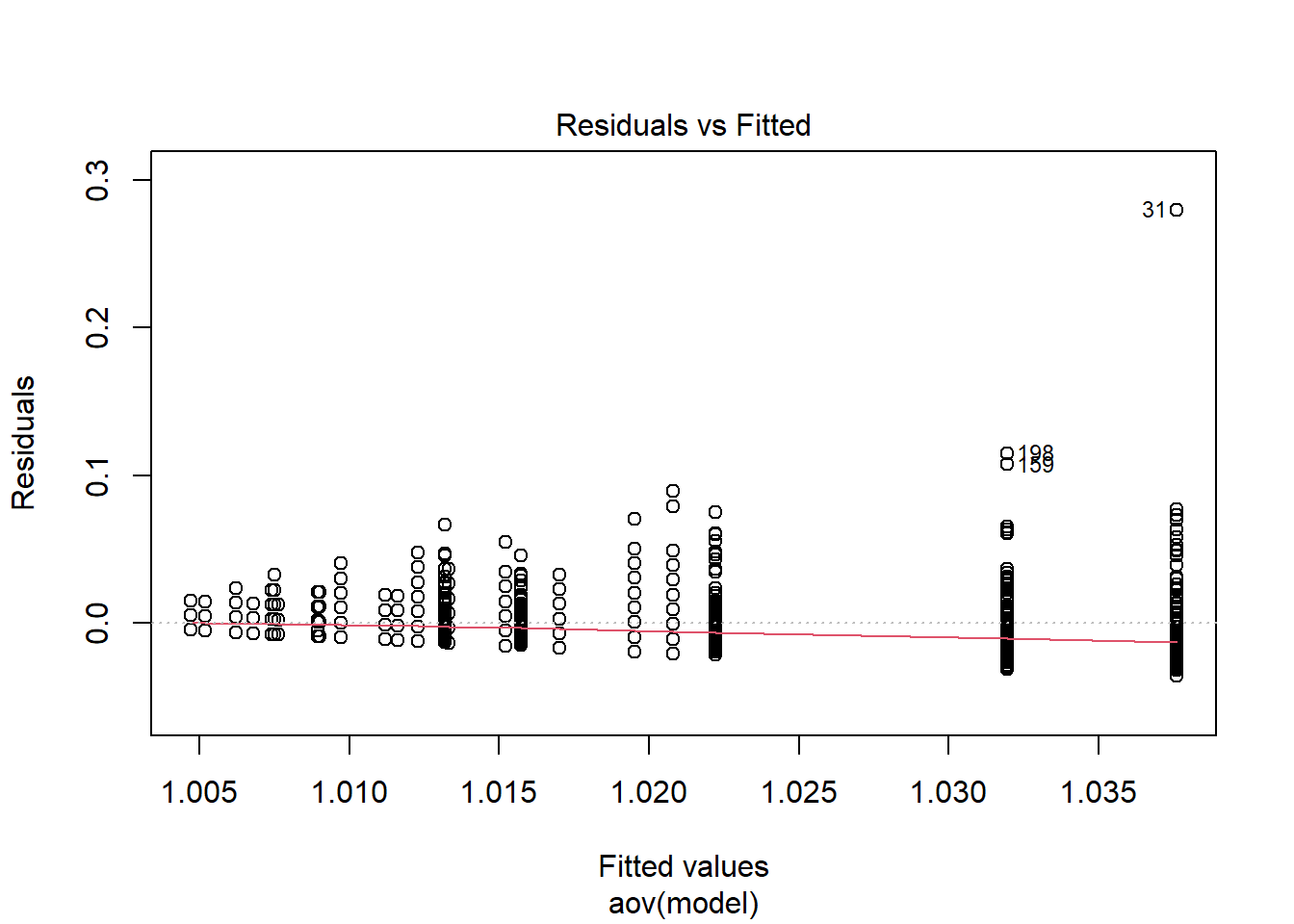


 Shapiro-Wilks Test of Normality of Residuals:

    Shapiro-Wilk normality test

data:  res
W = 0.7, p-value <0.0000000000000002


 K-S Test for Normality of Residuals:

Warning in ks.test(aov.out$residuals, "pnorm", alternative = "two.sided"): ties
should not be present for the Kolmogorov-Smirnov test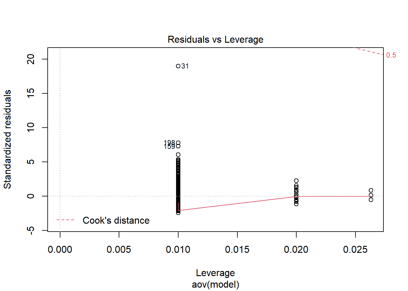


    One-sample Kolmogorov-Smirnov test

data:  aov.out$residuals
D = 0.5, p-value <0.0000000000000002
alternative hypothesis: two-sided

`stat_bin()` using `bins = 30`. Pick better value with `binwidth`.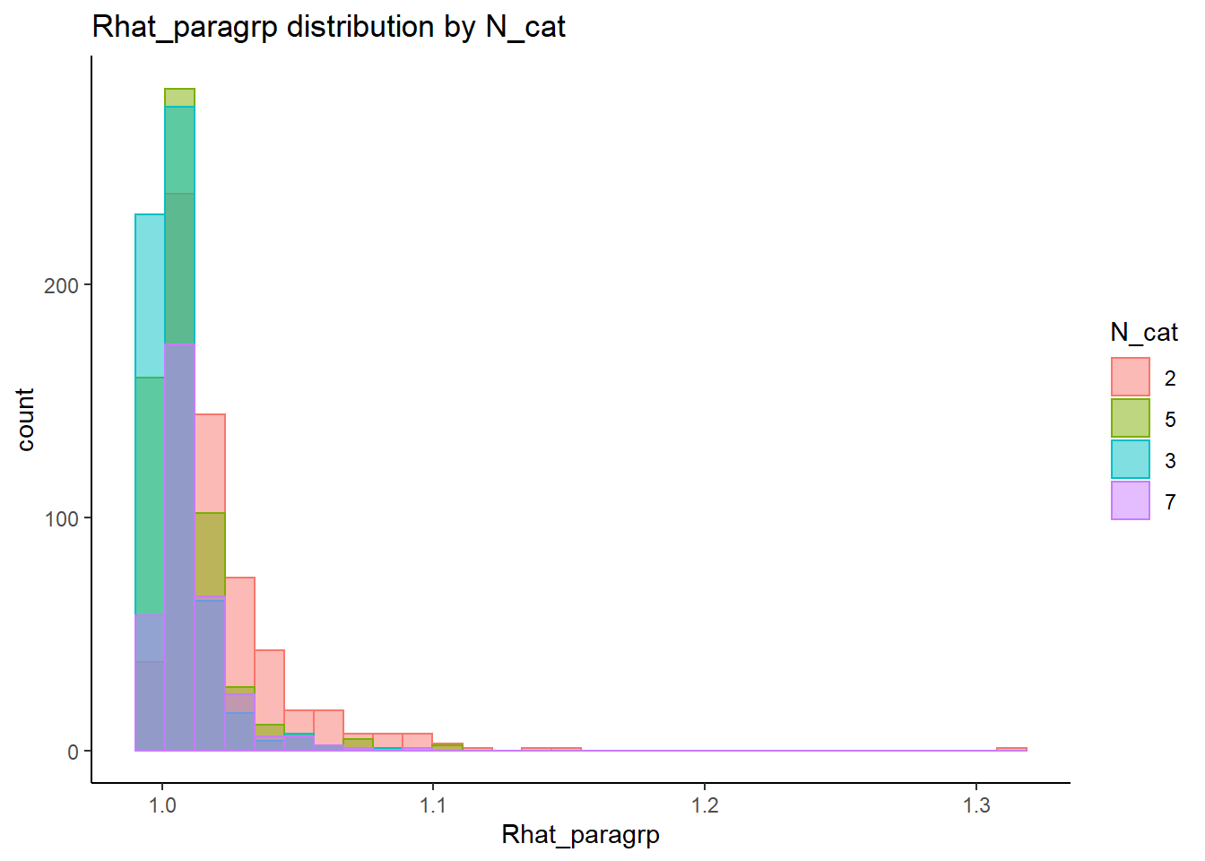

`stat_bin()` using `bins = 30`. Pick better value with `binwidth`.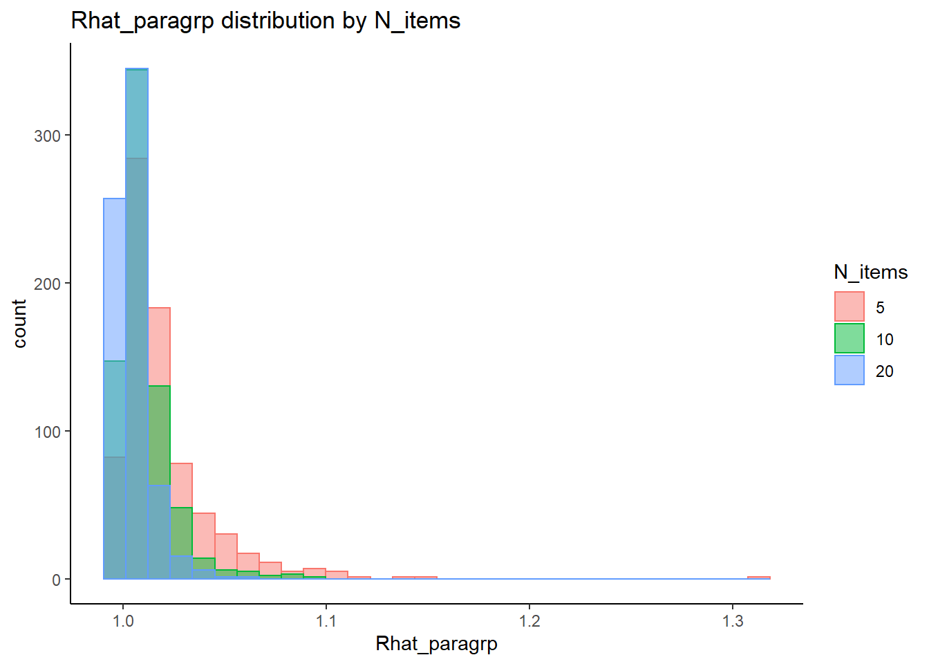

`stat_bin()` using `bins = 30`. Pick better value with `binwidth`.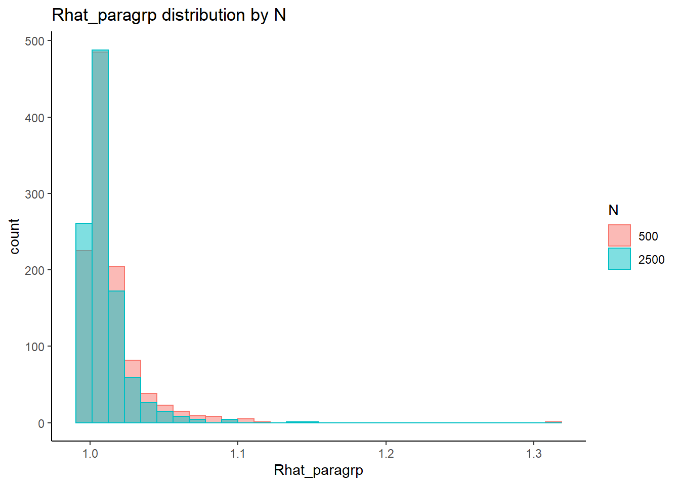


 ============================= 

 Tests of Homogeneity of Variance

 
 Levenes Test:  N_cat 
 
 
Levene's Test for Homogeneity of Variance (center = "mean")
        Df F value              Pr(>F)    
group    3    58.9 <0.0000000000000002 ***
      2134                                
---
Signif. codes:  0 '***' 0.001 '**' 0.01 '*' 0.05 '.' 0.1 ' ' 1

 
 Levenes Test:  N_items 
 
 
Levene's Test for Homogeneity of Variance (center = "mean")
        Df F value              Pr(>F)    
group    2    94.5 <0.0000000000000002 ***
      2135                                
---
Signif. codes:  0 '***' 0.001 '**' 0.01 '*' 0.05 '.' 0.1 ' ' 1

 
 Levenes Test:  N 
 
 
Levene's Test for Homogeneity of Variance (center = "mean")
        Df F value     Pr(>F)    
group    1    24.4 0.00000085 ***
      2136                       
---
Signif. codes:  0 '***' 0.001 '**' 0.01 '*' 0.05 '.' 0.1 ' ' 1

fit <- summary(aov(Rhat_paragrp ~ N_cat*N_items*N, data=conv_para_grp))
fit

                  Df Sum Sq Mean Sq F value               Pr(>F)    
N_cat              3  0.054  0.0180   82.10 < 0.0000000000000002 ***
N_items            2  0.071  0.0353  160.59 < 0.0000000000000002 ***
N                  1  0.005  0.0046   20.84      0.0000052682224 ***
N_cat:N_items      6  0.015  0.0025   11.28      0.0000000000019 ***
N_cat:N            3  0.002  0.0005    2.47                 0.06 .  
N_items:N          2  0.001  0.0003    1.29                 0.28    
N_cat:N_items:N    6  0.001  0.0001    0.49                 0.81    
Residuals       2114  0.464  0.0002                                 
---
Signif. codes:  0 '***' 0.001 '**' 0.01 '*' 0.05 '.' 0.1 ' ' 1

eta_est <- (fit[[1]]$`Sum Sq`/sum(fit[[1]]$`Sum Sq`))[1:7]
cbind(omega2(fit),p_omega2(fit), eta_est)

                omega^2 partial-omega^2  eta_est
N_cat            0.0874          0.1022 0.088504
N_items          0.1146          0.1299 0.115409
N                0.0071          0.0092 0.007490
N_cat:N_items    0.0222          0.0280 0.024326
N_cat:N          0.0016          0.0021 0.002668
N_items:N        0.0002          0.0003 0.000927
N_cat:N_items:N -0.0011         -0.0014 0.001065

saved_omega[7,] <- omega2(fit)
saved_eta[7,] <- eta_est

PID Relationship (\(\rho\))

conv_para_grp <- mydata %>%
  filter(parameter_group == "rho") %>%
  select(all_of(keep_cols)) %>%
  distinct()

## ANOVA on Rhat values
anova_assumptions_check(
  dat = conv_para_grp, outcome = 'Rhat_paragrp',
  factors = c('N_cat', 'N_items', 'N'),
  model = as.formula('Rhat_paragrp ~ N_cat*N_items*N'))


 ============================= 

 Tests and Plots of Normality: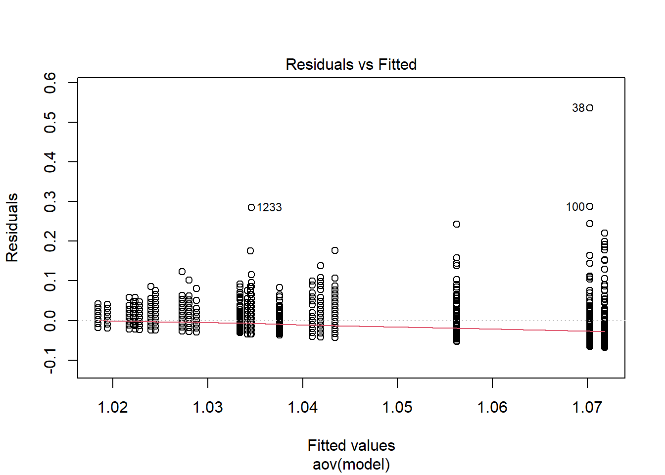


 Shapiro-Wilks Test of Normality of Residuals:

    Shapiro-Wilk normality test

data:  res
W = 0.8, p-value <0.0000000000000002


 K-S Test for Normality of Residuals:

Warning in ks.test(aov.out$residuals, "pnorm", alternative = "two.sided"): ties
should not be present for the Kolmogorov-Smirnov test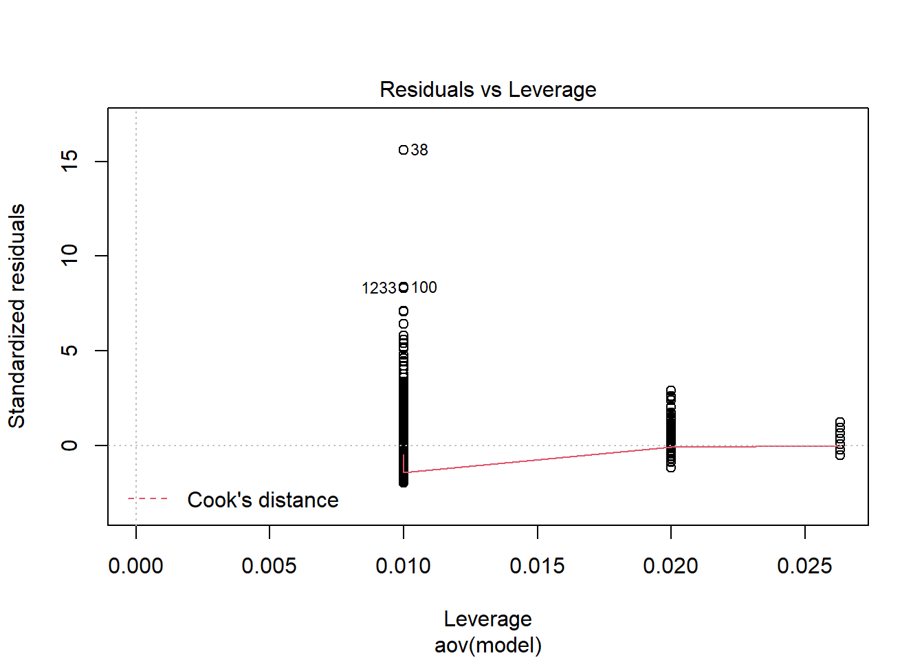


    One-sample Kolmogorov-Smirnov test

data:  aov.out$residuals
D = 0.5, p-value <0.0000000000000002
alternative hypothesis: two-sided

`stat_bin()` using `bins = 30`. Pick better value with `binwidth`.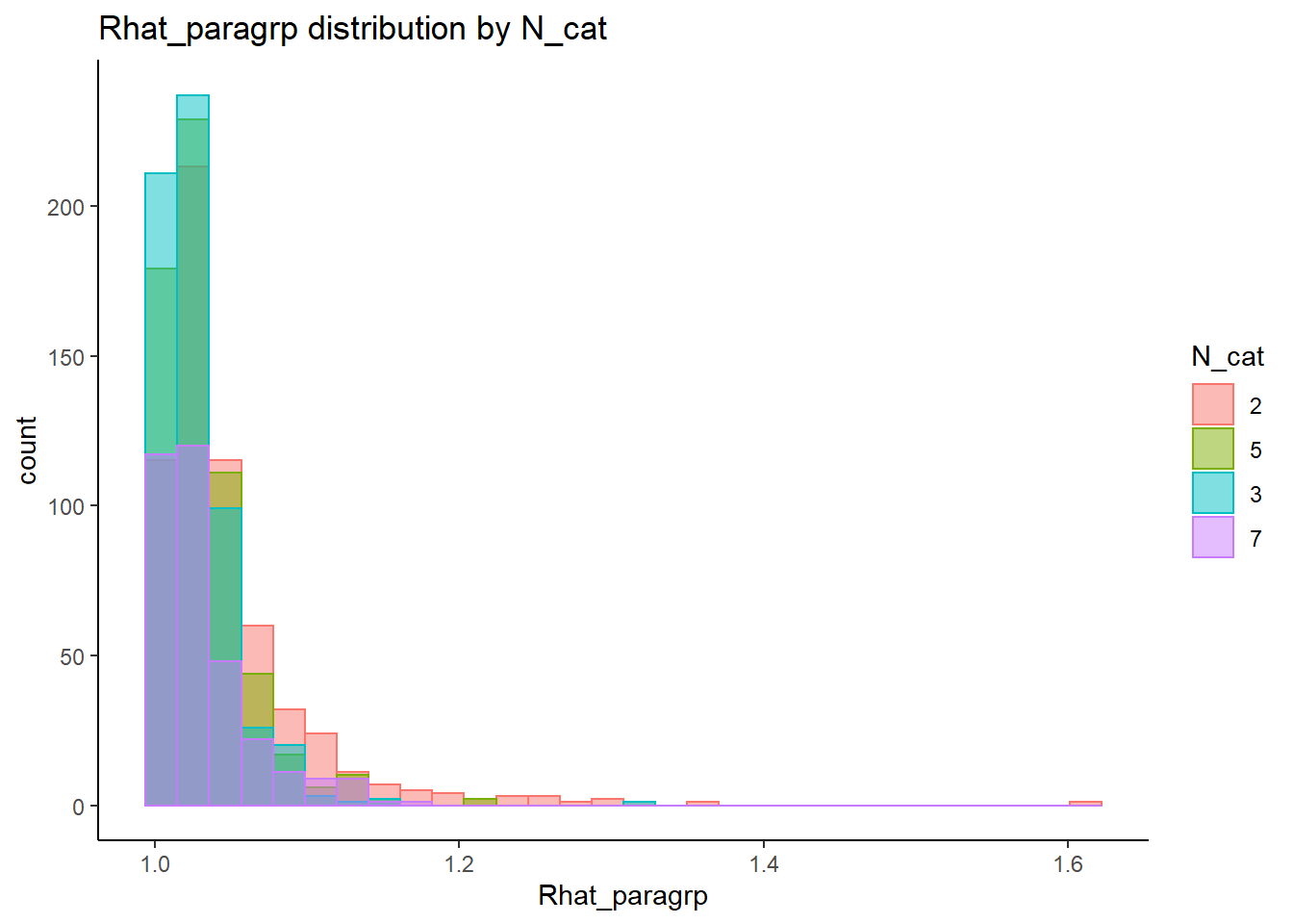

`stat_bin()` using `bins = 30`. Pick better value with `binwidth`.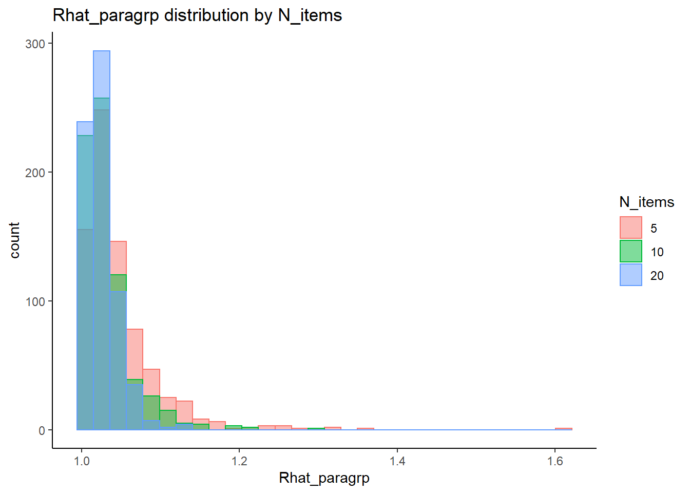

`stat_bin()` using `bins = 30`. Pick better value with `binwidth`.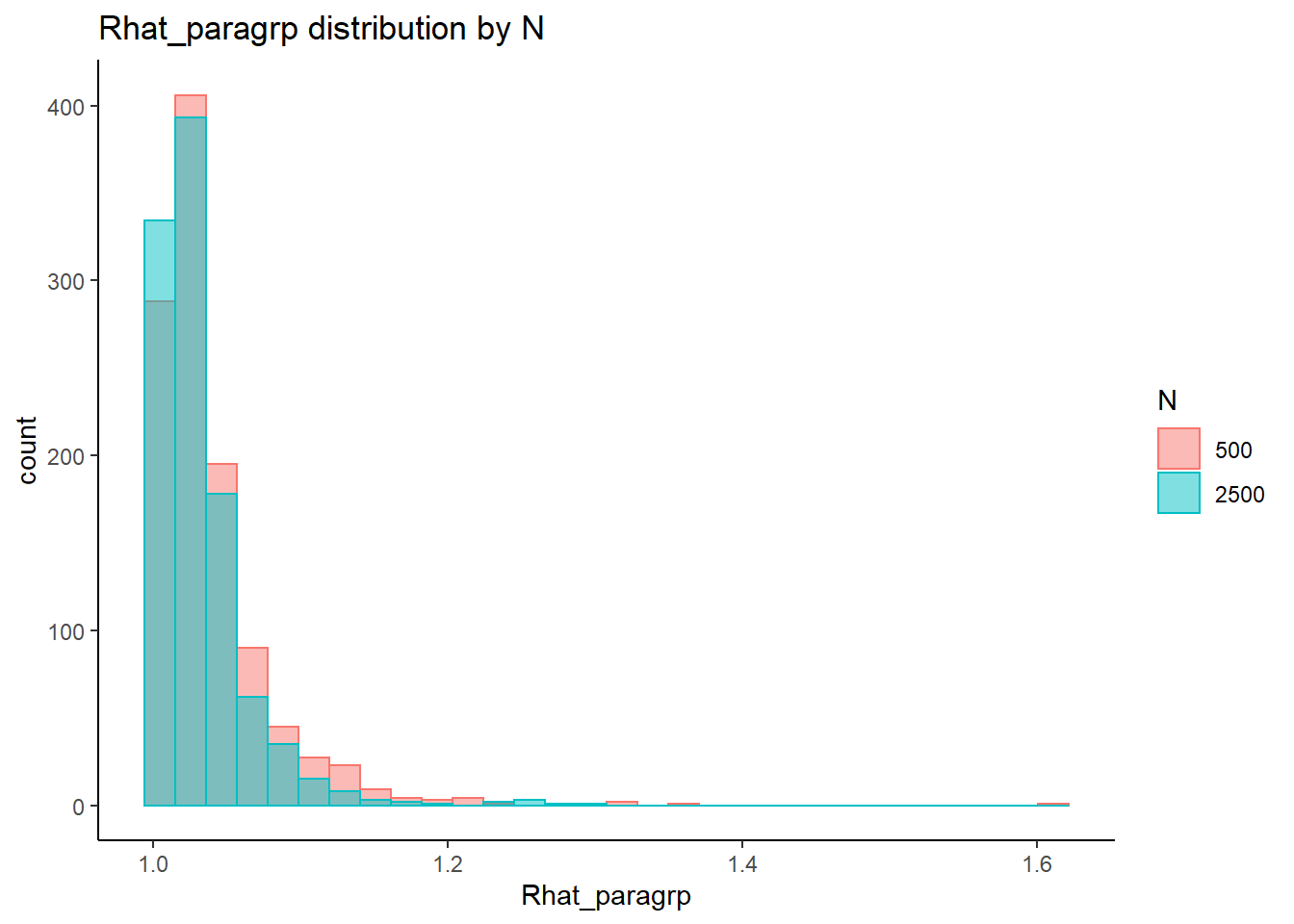


 ============================= 

 Tests of Homogeneity of Variance

 
 Levenes Test:  N_cat 
 
 
Levene's Test for Homogeneity of Variance (center = "mean")
        Df F value              Pr(>F)    
group    3    45.5 <0.0000000000000002 ***
      2134                                
---
Signif. codes:  0 '***' 0.001 '**' 0.01 '*' 0.05 '.' 0.1 ' ' 1

 
 Levenes Test:  N_items 
 
 
Levene's Test for Homogeneity of Variance (center = "mean")
        Df F value              Pr(>F)    
group    2      74 <0.0000000000000002 ***
      2135                                
---
Signif. codes:  0 '***' 0.001 '**' 0.01 '*' 0.05 '.' 0.1 ' ' 1

 
 Levenes Test:  N 
 
 
Levene's Test for Homogeneity of Variance (center = "mean")
        Df F value   Pr(>F)    
group    1    19.3 0.000012 ***
      2136                     
---
Signif. codes:  0 '***' 0.001 '**' 0.01 '*' 0.05 '.' 0.1 ' ' 1

fit <- summary(aov(Rhat_paragrp ~ N_cat*N_items*N, data=conv_para_grp))
fit

                  Df Sum Sq Mean Sq F value               Pr(>F)    
N_cat              3  0.162  0.0540   45.25 < 0.0000000000000002 ***
N_items            2  0.185  0.0925   77.44 < 0.0000000000000002 ***
N                  1  0.027  0.0273   22.88          0.000001846 ***
N_cat:N_items      6  0.053  0.0089    7.44          0.000000067 ***
N_cat:N            3  0.007  0.0024    1.99                0.114    
N_items:N          2  0.008  0.0039    3.24                0.039 *  
N_cat:N_items:N    6  0.010  0.0016    1.34                0.237    
Residuals       2114  2.524  0.0012                                 
---
Signif. codes:  0 '***' 0.001 '**' 0.01 '*' 0.05 '.' 0.1 ' ' 1

eta_est <- (fit[[1]]$`Sum Sq`/sum(fit[[1]]$`Sum Sq`))[1:7]
cbind(omega2(fit),p_omega2(fit), eta_est)

                omega^2 partial-omega^2 eta_est
N_cat            0.0532          0.0585 0.05447
N_items          0.0613          0.0667 0.06213
N                0.0088          0.0101 0.00918
N_cat:N_items    0.0155          0.0178 0.01791
N_cat:N          0.0012          0.0014 0.00239
N_items:N        0.0018          0.0021 0.00260
N_cat:N_items:N  0.0008          0.0009 0.00322

saved_omega[8,] <- omega2(fit)
saved_eta[8,] <- eta_est

Factor Reliability (\(\omega\))

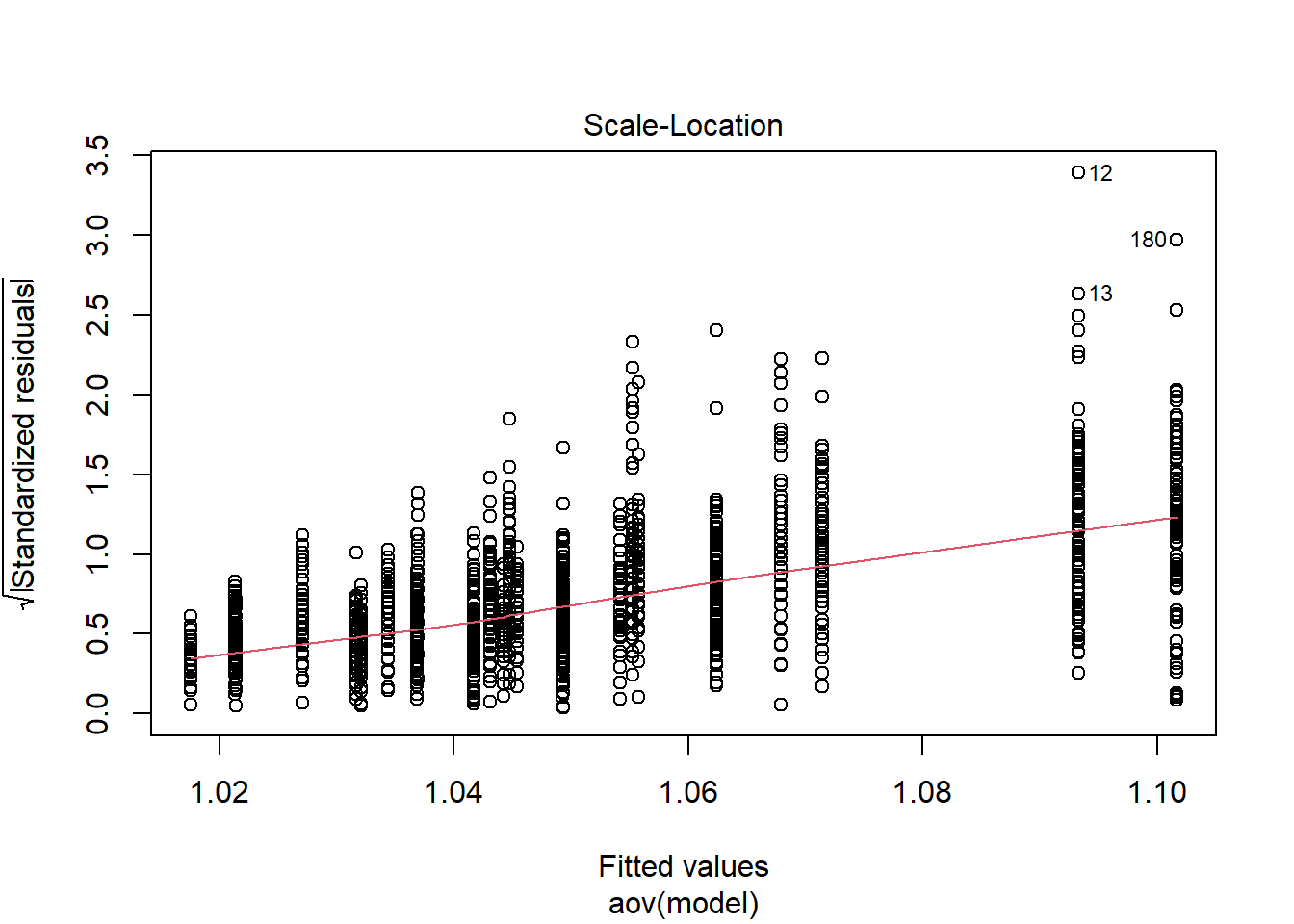
conv_para_grp <- mydata %>%
  filter(parameter_group == "omega") %>%
  select(all_of(keep_cols)) %>%
  distinct()

## ANOVA on Rhat values
anova_assumptions_check(
  dat = conv_para_grp, outcome = 'Rhat_paragrp',
  factors = c('N_cat', 'N_items', 'N'),
  model = as.formula('Rhat_paragrp ~ N_cat*N_items*N'))


 ============================= 

 Tests and Plots of Normality: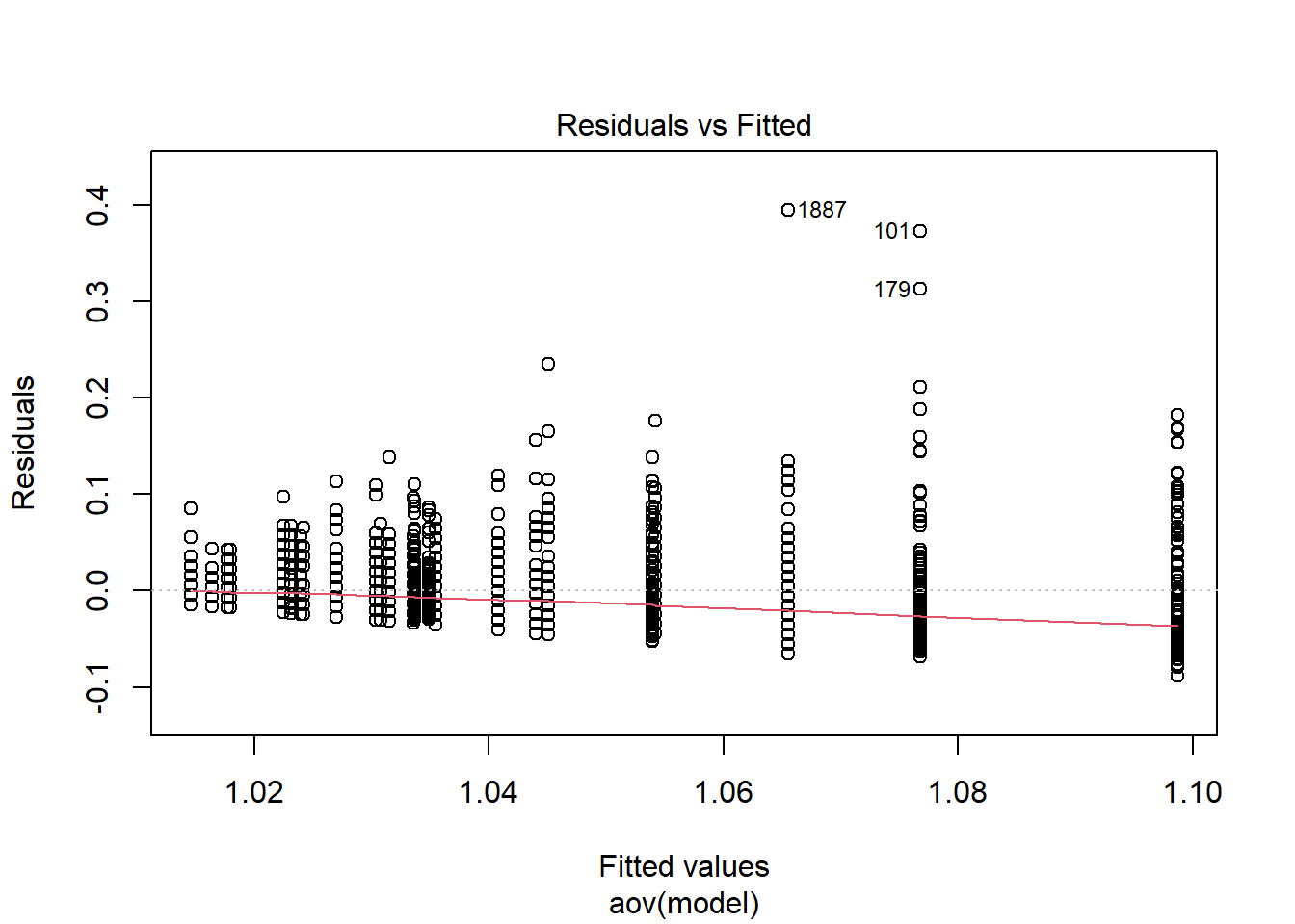


 Shapiro-Wilks Test of Normality of Residuals:

    Shapiro-Wilk normality test

data:  res
W = 0.8, p-value <0.0000000000000002


 K-S Test for Normality of Residuals:

Warning in ks.test(aov.out$residuals, "pnorm", alternative = "two.sided"): ties
should not be present for the Kolmogorov-Smirnov test


    One-sample Kolmogorov-Smirnov test

data:  aov.out$residuals
D = 0.5, p-value <0.0000000000000002
alternative hypothesis: two-sided

`stat_bin()` using `bins = 30`. Pick better value with `binwidth`.

`stat_bin()` using `bins = 30`. Pick better value with `binwidth`.

`stat_bin()` using `bins = 30`. Pick better value with `binwidth`.


 ============================= 

 Tests of Homogeneity of Variance

 
 Levenes Test:  N_cat 
 
 
Levene's Test for Homogeneity of Variance (center = "mean")
        Df F value              Pr(>F)    
group    3    67.1 <0.0000000000000002 ***
      2134                                
---
Signif. codes:  0 '***' 0.001 '**' 0.01 '*' 0.05 '.' 0.1 ' ' 1

 
 Levenes Test:  N_items 
 
 
Levene's Test for Homogeneity of Variance (center = "mean")
        Df F value              Pr(>F)    
group    2     124 <0.0000000000000002 ***
      2135                                
---
Signif. codes:  0 '***' 0.001 '**' 0.01 '*' 0.05 '.' 0.1 ' ' 1

 
 Levenes Test:  N 
 
 
Levene's Test for Homogeneity of Variance (center = "mean")
        Df F value           Pr(>F)    
group    1    55.7 0.00000000000012 ***
      2136                             
---
Signif. codes:  0 '***' 0.001 '**' 0.01 '*' 0.05 '.' 0.1 ' ' 1

fit <- summary(aov(Rhat_paragrp ~ N_cat*N_items*N, data=conv_para_grp))
fit

                  Df Sum Sq Mean Sq F value               Pr(>F)    
N_cat              3  0.311  0.1036   80.46 < 0.0000000000000002 ***
N_items            2  0.381  0.1904  147.84 < 0.0000000000000002 ***
N                  1  0.087  0.0874   67.85  0.00000000000000031 ***
N_cat:N_items      6  0.124  0.0206   16.01 < 0.0000000000000002 ***
N_cat:N            3  0.007  0.0024    1.89              0.12980    
N_items:N          2  0.023  0.0113    8.78              0.00016 ***
N_cat:N_items:N    6  0.005  0.0008    0.58              0.74283    
Residuals       2114  2.723  0.0013                                 
---
Signif. codes:  0 '***' 0.001 '**' 0.01 '*' 0.05 '.' 0.1 ' ' 1

eta_est <- (fit[[1]]$`Sum Sq`/sum(fit[[1]]$`Sum Sq`))[1:7]
cbind(omega2(fit),p_omega2(fit), eta_est)

                omega^2 partial-omega^2 eta_est
N_cat            0.0839          0.1003 0.08494
N_items          0.1033          0.1208 0.10405
N                0.0235          0.0303 0.02387
N_cat:N_items    0.0317          0.0404 0.03380
N_cat:N          0.0009          0.0012 0.00199
N_items:N        0.0055          0.0072 0.00618
N_cat:N_items:N -0.0009         -0.0012 0.00123

saved_omega[9,] <- omega2(fit)
saved_eta[9,] <- eta_est

Manuscript Tables and Figures (latex formated)

Tables

print(
  xtable(
    t(saved_omega)
    , caption = c("Effect of design factors on relative bias estimates: omega2")
    ,align = "lrrrrrrrrr", digits = 3
  ),
  include.rownames=T,
  booktabs=T
)

% latex table generated in R 4.0.5 by xtable 1.8-4 package
% Sun Feb 13 14:28:59 2022
\begin{table}[ht]
\centering
\begin{tabular}{lrrrrrrrrr}
  \toprule
 & lambda & tau & theta & beta\_lrt & sigma\_lrt & sigma\_s & sigma\_ts & rho & omega \\ 
  \midrule
N\_cat & 0.189 & 0.242 & 0.186 & 0.136 & 0.168 & 0.068 & 0.087 & 0.053 & 0.084 \\ 
  N\_items & 0.222 & 0.104 & 0.225 & 0.211 & 0.123 & 0.167 & 0.115 & 0.061 & 0.103 \\ 
  N & 0.021 & 0.064 & 0.042 & 0.001 & 0.020 & -0.000 & 0.007 & 0.009 & 0.024 \\ 
  N\_cat:N\_items & 0.053 & 0.026 & 0.076 & 0.053 & 0.132 & 0.031 & 0.022 & 0.015 & 0.032 \\ 
  N\_cat:N & 0.002 & 0.003 & 0.001 & 0.000 & 0.017 & -0.001 & 0.002 & 0.001 & 0.001 \\ 
  N\_items:N & 0.001 & 0.020 & 0.009 & 0.000 & 0.016 & 0.001 & 0.000 & 0.002 & 0.005 \\ 
  N\_cat:N\_items:N & 0.012 & 0.000 & 0.001 & 0.001 & 0.005 & -0.001 & -0.001 & 0.001 & -0.001 \\ 
   \bottomrule
\end{tabular}
\caption{Effect of design factors on relative bias estimates: omega2} 
\end{table}

print(
  xtable(
    t(saved_eta)
    , caption = c("Effect of design factors on relative bias estimates: eta2")
    ,align = "lrrrrrrrrr", digits = 3
  ),
  include.rownames=T,
  booktabs=T
)

% latex table generated in R 4.0.5 by xtable 1.8-4 package
% Sun Feb 13 14:28:59 2022
\begin{table}[ht]
\centering
\begin{tabular}{lrrrrrrrrr}
  \toprule
 & lambda & tau & theta & beta\_lrt & sigma\_lrt & sigma\_s & sigma\_ts & rho & omega \\ 
  \midrule
N\_cat & 0.189 & 0.243 & 0.186 & 0.137 & 0.168 & 0.069 & 0.089 & 0.054 & 0.085 \\ 
  N\_items & 0.222 & 0.105 & 0.225 & 0.212 & 0.124 & 0.168 & 0.115 & 0.062 & 0.104 \\ 
  N & 0.021 & 0.065 & 0.042 & 0.001 & 0.020 & 0.000 & 0.007 & 0.009 & 0.024 \\ 
  N\_cat:N\_items & 0.054 & 0.027 & 0.077 & 0.055 & 0.133 & 0.033 & 0.024 & 0.018 & 0.034 \\ 
  N\_cat:N & 0.002 & 0.004 & 0.002 & 0.001 & 0.018 & 0.000 & 0.003 & 0.002 & 0.002 \\ 
  N\_items:N & 0.001 & 0.021 & 0.010 & 0.001 & 0.017 & 0.002 & 0.001 & 0.003 & 0.006 \\ 
  N\_cat:N\_items:N & 0.014 & 0.002 & 0.002 & 0.003 & 0.007 & 0.001 & 0.001 & 0.003 & 0.001 \\ 
   \bottomrule
\end{tabular}
\caption{Effect of design factors on relative bias estimates: eta2} 
\end{table}

keep_cols <- c("condition", "iter", "N", "N_items", "N_cat", "parameter_group", "Rhat_paragrp", "converge_paragrp", "converge_proportion_paragrp")

tbl_dat <- mydata %>%
  select(all_of(keep_cols)) %>%
  filter(
    !is.na(parameter_group)
    , parameter_group != "lambda (STD)"
  ) %>%
  distinct() %>%
  mutate(
    prop_con = ifelse(converge_proportion_paragrp > 0.5, ">50% Converged", "<=50% Converged")
  )


# get average Rhat and SD for each condition and parameter group
sum_tab <- tbl_dat %>%
  group_by(N_cat, N_items, N, parameter_group) %>%
  summarise(
    AvgRhat = mean(Rhat_paragrp),
    SDRhat = sd(Rhat_paragrp),
    AvgPropConv = mean(converge_proportion_paragrp)
  )

`summarise()` has grouped output by 'N_cat', 'N_items', 'N'. You can override using the `.groups` argument.

# table 1: 2 category data
T1 <- sum_tab %>%
  filter(N_cat == 2) %>%
  pivot_wider(
    id_cols = c("parameter_group", "N")
    , names_from = "N_items"
    , values_from = all_of(c("AvgRhat", "SDRhat", "AvgPropConv"))
  ) %>%
  arrange(.,parameter_group)
# reordering of rows to more logical for presentation
T1 <- T1[c(3:4, 15:18, 1:2, 5:8, 13:14, 11:12, 9:10) ,]
print(
  xtable(
    T1
    , caption = c("Posterior convergence by Rhat summary: Dichotomous items")
    ,align = "llrrrrrrrrrr"
  ),
  include.rownames=F,
  booktabs=T
)

% latex table generated in R 4.0.5 by xtable 1.8-4 package
% Sun Feb 13 14:29:00 2022
\begin{table}[ht]
\centering
\begin{tabular}{lrrrrrrrrrr}
  \toprule
parameter\_group & N & AvgRhat\_5 & AvgRhat\_10 & AvgRhat\_20 & SDRhat\_5 & SDRhat\_10 & SDRhat\_20 & AvgPropConv\_5 & AvgPropConv\_10 & AvgPropConv\_20 \\ 
  \midrule
lambda & 500 & 1.09 & 1.06 & 1.04 & 0.05 & 0.02 & 0.01 & 0.68 & 0.85 & 0.95 \\ 
  lambda & 2500 & 1.10 & 1.05 & 1.03 & 0.05 & 0.01 & 0.00 & 0.65 & 0.90 & 0.97 \\ 
  tau & 500 & 1.03 & 1.02 & 1.01 & 0.02 & 0.01 & 0.00 & 0.96 & 0.98 & 1.00 \\ 
  tau & 2500 & 1.02 & 1.01 & 1.01 & 0.01 & 0.00 & 0.00 & 0.98 & 1.00 & 1.00 \\ 
  theta & 500 & 1.14 & 1.08 & 1.05 & 0.07 & 0.03 & 0.01 & 0.50 & 0.76 & 0.92 \\ 
  theta & 2500 & 1.11 & 1.05 & 1.03 & 0.05 & 0.01 & 0.01 & 0.62 & 0.89 & 0.97 \\ 
  beta\_lrt & 500 & 1.07 & 1.04 & 1.02 & 0.04 & 0.02 & 0.01 & 0.80 & 0.93 & 0.99 \\ 
  beta\_lrt & 2500 & 1.07 & 1.03 & 1.02 & 0.04 & 0.01 & 0.01 & 0.80 & 0.97 & 1.00 \\ 
  sigma\_lrt & 500 & 1.01 & 1.00 & 1.00 & 0.01 & 0.01 & 0.00 & 0.97 & 1.00 & 1.00 \\ 
  sigma\_lrt & 2500 & 1.01 & 1.00 & 1.00 & 0.01 & 0.00 & 0.00 & 0.99 & 1.00 & 1.00 \\ 
  sigma\_s & 500 & 1.02 & 1.01 & 1.00 & 0.02 & 0.01 & 0.00 & 0.99 & 1.00 & 1.00 \\ 
  sigma\_s & 2500 & 1.02 & 1.01 & 1.00 & 0.02 & 0.01 & 0.00 & 0.97 & 1.00 & 1.00 \\ 
  sigma\_st & 500 & 1.04 & 1.02 & 1.01 & 0.04 & 0.02 & 0.01 & 0.95 & 1.00 & 1.00 \\ 
  sigma\_st & 2500 & 1.03 & 1.02 & 1.01 & 0.03 & 0.01 & 0.01 & 0.98 & 1.00 & 1.00 \\ 
  rho & 500 & 1.07 & 1.06 & 1.04 & 0.08 & 0.05 & 0.02 & 0.82 & 0.85 & 0.97 \\ 
  rho & 2500 & 1.07 & 1.03 & 1.02 & 0.07 & 0.03 & 0.01 & 0.80 & 0.97 & 1.00 \\ 
  omega & 500 & 1.10 & 1.05 & 1.03 & 0.07 & 0.04 & 0.03 & 0.63 & 0.88 & 0.96 \\ 
  omega & 2500 & 1.08 & 1.03 & 1.02 & 0.08 & 0.02 & 0.02 & 0.78 & 0.97 & 1.00 \\ 
   \bottomrule
\end{tabular}
\caption{Posterior convergence by Rhat summary: Dichotomous items} 
\end{table}

# table 2: 5 category data
T2 <- sum_tab %>%
  filter(N_cat == 5) %>%
  pivot_wider(
    id_cols = c("parameter_group", "N")
    , names_from = "N_items"
    , values_from = all_of(c("AvgRhat", "SDRhat", "AvgPropConv"))
  ) %>%
  arrange(.,parameter_group)
# reordering of rows to more logical for presentation
T2 <- T2[c(3:4, 15:18, 1:2, 5:8, 13:14, 11:12, 9:10) ,]
print(
  xtable(
    T2
    , caption = c("Posterior convergence by Rhat summary: Five category items")
    ,align = "llrrrrrrrrrr"
  ),
  include.rownames=F,
  booktabs=T
)

% latex table generated in R 4.0.5 by xtable 1.8-4 package
% Sun Feb 13 14:29:00 2022
\begin{table}[ht]
\centering
\begin{tabular}{lrrrrrrrrrr}
  \toprule
parameter\_group & N & AvgRhat\_5 & AvgRhat\_10 & AvgRhat\_20 & SDRhat\_5 & SDRhat\_10 & SDRhat\_20 & AvgPropConv\_5 & AvgPropConv\_10 & AvgPropConv\_20 \\ 
  \midrule
lambda & 500 & 1.07 & 1.04 & 1.04 & 0.03 & 0.01 & 0.01 & 0.78 & 0.92 & 0.94 \\ 
  lambda & 2500 & 1.04 & 1.03 & 1.03 & 0.02 & 0.01 & 0.01 & 0.91 & 0.96 & 0.97 \\ 
  tau & 500 & 1.02 & 1.02 & 1.02 & 0.01 & 0.00 & 0.00 & 0.97 & 0.99 & 1.00 \\ 
  tau & 2500 & 1.02 & 1.02 & 1.02 & 0.01 & 0.00 & 0.00 & 1.00 & 1.00 & 1.00 \\ 
  theta & 500 & 1.08 & 1.05 & 1.04 & 0.04 & 0.01 & 0.01 & 0.73 & 0.91 & 0.94 \\ 
  theta & 2500 & 1.05 & 1.03 & 1.03 & 0.02 & 0.01 & 0.01 & 0.90 & 0.96 & 0.97 \\ 
  beta\_lrt & 500 & 1.03 & 1.02 & 1.01 & 0.02 & 0.02 & 0.01 & 0.93 & 0.98 & 1.00 \\ 
  beta\_lrt & 2500 & 1.03 & 1.02 & 1.01 & 0.02 & 0.01 & 0.01 & 0.98 & 1.00 & 1.00 \\ 
  sigma\_lrt & 500 & 1.00 & 1.00 & 1.00 & 0.00 & 0.00 & 0.00 & 1.00 & 1.00 & 1.00 \\ 
  sigma\_lrt & 2500 & 1.00 & 1.00 & 1.00 & 0.00 & 0.00 & 0.00 & 1.00 & 1.00 & 1.00 \\ 
  sigma\_s & 500 & 1.01 & 1.00 & 1.00 & 0.01 & 0.01 & 0.00 & 1.00 & 1.00 & 1.00 \\ 
  sigma\_s & 2500 & 1.01 & 1.00 & 1.00 & 0.01 & 0.01 & 0.00 & 1.00 & 1.00 & 1.00 \\ 
  sigma\_st & 500 & 1.02 & 1.01 & 1.01 & 0.02 & 0.01 & 0.01 & 0.98 & 1.00 & 1.00 \\ 
  sigma\_st & 2500 & 1.02 & 1.01 & 1.01 & 0.01 & 0.01 & 0.01 & 1.00 & 1.00 & 1.00 \\ 
  rho & 500 & 1.04 & 1.03 & 1.03 & 0.04 & 0.03 & 0.02 & 0.91 & 0.94 & 0.98 \\ 
  rho & 2500 & 1.03 & 1.02 & 1.02 & 0.03 & 0.02 & 0.02 & 0.97 & 1.00 & 1.00 \\ 
  omega & 500 & 1.05 & 1.04 & 1.03 & 0.04 & 0.03 & 0.03 & 0.87 & 0.95 & 0.98 \\ 
  omega & 2500 & 1.03 & 1.03 & 1.02 & 0.03 & 0.02 & 0.02 & 0.99 & 0.97 & 0.99 \\ 
   \bottomrule
\end{tabular}
\caption{Posterior convergence by Rhat summary: Five category items} 
\end{table}

# table 3: 3 category data
T3 <- sum_tab %>%
  filter(N_cat == 3) %>%
  pivot_wider(
    id_cols = c("parameter_group", "N")
    , names_from = "N_items"
    , values_from = all_of(c("AvgRhat", "SDRhat", "AvgPropConv"))
  ) %>%
  arrange(.,parameter_group)
# reordering of rows to more logical for presentation
T3 <- T3[c(3:4, 15:18, 1:2, 5:8, 13:14, 11:12, 9:10) ,]
print(
  xtable(
    T3
    , caption = c("Posterior convergence by Rhat summary: Three category items")
    ,align = "llrrrrrrrrrr"
  ),
  include.rownames=F,
  booktabs=T
)

% latex table generated in R 4.0.5 by xtable 1.8-4 package
% Sun Feb 13 14:29:00 2022
\begin{table}[ht]
\centering
\begin{tabular}{lrrrrrrrrrr}
  \toprule
parameter\_group & N & AvgRhat\_5 & AvgRhat\_10 & AvgRhat\_20 & SDRhat\_5 & SDRhat\_10 & SDRhat\_20 & AvgPropConv\_5 & AvgPropConv\_10 & AvgPropConv\_20 \\ 
  \midrule
lambda & 500 & 1.06 & 1.03 & 1.02 & 0.03 & 0.01 & 0.00 & 0.87 & 0.98 & 0.99 \\ 
  lambda & 2500 & 1.04 & 1.02 & 1.02 & 0.01 & 0.01 & 0.00 & 0.95 & 0.99 & 1.00 \\ 
  tau & 500 & 1.02 & 1.01 & 1.01 & 0.01 & 0.00 & 0.00 & 0.98 & 1.00 & 1.00 \\ 
  tau & 2500 & 1.01 & 1.01 & 1.01 & 0.00 & 0.00 & 0.00 & 1.00 & 1.00 & 1.00 \\ 
  theta & 500 & 1.07 & 1.03 & 1.02 & 0.04 & 0.01 & 0.00 & 0.80 & 0.98 & 0.99 \\ 
  theta & 2500 & 1.04 & 1.02 & 1.02 & 0.02 & 0.01 & 0.00 & 0.93 & 0.99 & 1.00 \\ 
  beta\_lrt & 500 & 1.03 & 1.02 & 1.01 & 0.02 & 0.01 & 0.01 & 0.96 & 1.00 & 1.00 \\ 
  beta\_lrt & 2500 & 1.03 & 1.02 & 1.01 & 0.02 & 0.01 & 0.01 & 0.99 & 1.00 & 1.00 \\ 
  sigma\_lrt & 500 & 1.00 & 1.00 & 1.00 & 0.00 & 0.00 & 0.00 & 1.00 & 1.00 & 1.00 \\ 
  sigma\_lrt & 2500 & 1.00 & 1.00 & 1.00 & 0.00 & 0.00 & 0.00 & 1.00 & 1.00 & 1.00 \\ 
  sigma\_s & 500 & 1.01 & 1.00 & 1.00 & 0.01 & 0.01 & 0.00 & 1.00 & 1.00 & 1.00 \\ 
  sigma\_s & 2500 & 1.01 & 1.00 & 1.00 & 0.01 & 0.01 & 0.00 & 1.00 & 1.00 & 1.00 \\ 
  sigma\_st & 500 & 1.01 & 1.01 & 1.01 & 0.01 & 0.01 & 0.01 & 1.00 & 1.00 & 1.00 \\ 
  sigma\_st & 2500 & 1.01 & 1.01 & 1.00 & 0.01 & 0.01 & 0.01 & 1.00 & 1.00 & 1.00 \\ 
  rho & 500 & 1.03 & 1.03 & 1.02 & 0.04 & 0.02 & 0.02 & 0.97 & 0.99 & 0.99 \\ 
  rho & 2500 & 1.03 & 1.02 & 1.02 & 0.02 & 0.02 & 0.01 & 0.98 & 1.00 & 1.00 \\ 
  omega & 500 & 1.05 & 1.02 & 1.02 & 0.04 & 0.01 & 0.01 & 0.89 & 1.00 & 1.00 \\ 
  omega & 2500 & 1.02 & 1.02 & 1.01 & 0.02 & 0.01 & 0.02 & 1.00 & 1.00 & 0.99 \\ 
   \bottomrule
\end{tabular}
\caption{Posterior convergence by Rhat summary: Three category items} 
\end{table}

# table 4: 7 category data
T4 <- sum_tab %>%
  filter(N_cat == 7) %>%
  pivot_wider(
    id_cols = c("parameter_group", "N")
    , names_from = "N_items"
    , values_from = all_of(c("AvgRhat", "SDRhat", "AvgPropConv"))
  ) %>%
  arrange(.,parameter_group)
# reordering of rows to more logical for presentation
T4 <- T4[c(3:4, 15:18, 1:2, 5:8, 13:14, 11:12, 9:10) ,]
print(
  xtable(
    T4
    , caption = c("Posterior convergence by Rhat summary: Seven category items")
    ,align = "llrrrrrrrrrr"
  ),
  include.rownames=F,
  booktabs=T
)

% latex table generated in R 4.0.5 by xtable 1.8-4 package
% Sun Feb 13 14:29:00 2022
\begin{table}[ht]
\centering
\begin{tabular}{lrrrrrrrrrr}
  \toprule
parameter\_group & N & AvgRhat\_5 & AvgRhat\_10 & AvgRhat\_20 & SDRhat\_5 & SDRhat\_10 & SDRhat\_20 & AvgPropConv\_5 & AvgPropConv\_10 & AvgPropConv\_20 \\ 
  \midrule
lambda & 500 & 1.07 & 1.05 & 1.05 & 0.03 & 0.02 & 0.01 & 0.78 & 0.85 & 0.88 \\ 
  lambda & 2500 & 1.06 & 1.05 & 1.04 & 0.02 & 0.01 & 0.01 & 0.83 & 0.90 & 0.92 \\ 
  tau & 500 & 1.03 & 1.02 & 1.02 & 0.01 & 0.00 & 0.00 & 0.95 & 0.99 & 0.99 \\ 
  tau & 2500 & 1.02 & 1.02 & 1.02 & 0.01 & 0.00 & 0.00 & 0.99 & 1.00 & 1.00 \\ 
  theta & 500 & 1.08 & 1.06 & 1.05 & 0.03 & 0.02 & 0.01 & 0.75 & 0.84 & 0.86 \\ 
  theta & 2500 & 1.06 & 1.05 & 1.04 & 0.03 & 0.01 & 0.01 & 0.82 & 0.90 & 0.92 \\ 
  beta\_lrt & 500 & 1.03 & 1.02 & 1.01 & 0.02 & 0.01 & 0.01 & 0.96 & 0.99 & 1.00 \\ 
  beta\_lrt & 2500 & 1.03 & 1.02 & 1.01 & 0.02 & 0.01 & 0.01 & 0.95 & 0.99 & 1.00 \\ 
  sigma\_lrt & 500 & 1.00 & 1.00 & 1.00 & 0.00 & 0.00 & 0.00 & 1.00 & 1.00 & 1.00 \\ 
  sigma\_lrt & 2500 & 1.00 & 1.00 & 1.00 & 0.00 & 0.00 & 0.00 & 1.00 & 1.00 & 1.00 \\ 
  sigma\_s & 500 & 1.01 & 1.00 & 1.00 & 0.01 & 0.01 & 0.00 & 1.00 & 1.00 & 1.00 \\ 
  sigma\_s & 2500 & 1.01 & 1.00 & 1.00 & 0.01 & 0.01 & 0.00 & 1.00 & 1.00 & 1.00 \\ 
  sigma\_st & 500 & 1.02 & 1.01 & 1.01 & 0.02 & 0.01 & 0.01 & 1.00 & 1.00 & 1.00 \\ 
  sigma\_st & 2500 & 1.02 & 1.01 & 1.01 & 0.01 & 0.01 & 0.01 & 1.00 & 1.00 & 1.00 \\ 
  rho & 500 & 1.04 & 1.03 & 1.02 & 0.04 & 0.02 & 0.01 & 0.87 & 0.98 & 1.00 \\ 
  rho & 2500 & 1.04 & 1.02 & 1.02 & 0.03 & 0.02 & 0.01 & 0.90 & 0.98 & 1.00 \\ 
  omega & 500 & 1.07 & 1.04 & 1.03 & 0.06 & 0.03 & 0.03 & 0.81 & 0.92 & 0.98 \\ 
  omega & 2500 & 1.04 & 1.03 & 1.02 & 0.04 & 0.02 & 0.02 & 0.86 & 0.98 & 1.00 \\ 
   \bottomrule
\end{tabular}
\caption{Posterior convergence by Rhat summary: Seven category items} 
\end{table}

sessionInfo()

R version 4.0.5 (2021-03-31)
Platform: x86_64-w64-mingw32/x64 (64-bit)
Running under: Windows 10 x64 (build 22000)

Matrix products: default

locale:
[1] LC_COLLATE=English_United States.1252 
[2] LC_CTYPE=English_United States.1252   
[3] LC_MONETARY=English_United States.1252
[4] LC_NUMERIC=C                          
[5] LC_TIME=English_United States.1252    

attached base packages:
[1] stats     graphics  grDevices utils     datasets  methods   base     

other attached packages:
 [1] car_3.0-10           carData_3.0-4        mvtnorm_1.1-1       
 [4] LaplacesDemon_16.1.4 runjags_2.2.0-2      lme4_1.1-26         
 [7] Matrix_1.3-2         sirt_3.9-4           R2jags_0.6-1        
[10] rjags_4-12           eRm_1.0-2            diffIRT_1.5         
[13] statmod_1.4.35       xtable_1.8-4         kableExtra_1.3.4    
[16] lavaan_0.6-7         polycor_0.7-10       bayesplot_1.8.0     
[19] ggmcmc_1.5.1.1       coda_0.19-4          data.table_1.14.0   
[22] patchwork_1.1.1      forcats_0.5.1        stringr_1.4.0       
[25] dplyr_1.0.5          purrr_0.3.4          readr_1.4.0         
[28] tidyr_1.1.3          tibble_3.1.0         ggplot2_3.3.5       
[31] tidyverse_1.3.0      workflowr_1.6.2     

loaded via a namespace (and not attached):
 [1] minqa_1.2.4        TAM_3.5-19         colorspace_2.0-0   rio_0.5.26        
 [5] ellipsis_0.3.1     ggridges_0.5.3     rprojroot_2.0.2    fs_1.5.0          
 [9] rstudioapi_0.13    farver_2.1.0       fansi_0.4.2        lubridate_1.7.10  
[13] xml2_1.3.2         splines_4.0.5      mnormt_2.0.2       knitr_1.31        
[17] jsonlite_1.7.2     nloptr_1.2.2.2     broom_0.7.5        dbplyr_2.1.0      
[21] compiler_4.0.5     httr_1.4.2         backports_1.2.1    assertthat_0.2.1  
[25] cli_2.3.1          later_1.1.0.1      htmltools_0.5.1.1  tools_4.0.5       
[29] gtable_0.3.0       glue_1.4.2         Rcpp_1.0.7         cellranger_1.1.0  
[33] jquerylib_0.1.3    vctrs_0.3.6        svglite_2.0.0      nlme_3.1-152      
[37] psych_2.0.12       xfun_0.21          ps_1.6.0           openxlsx_4.2.3    
[41] rvest_1.0.0        lifecycle_1.0.0    MASS_7.3-53.1      scales_1.1.1      
[45] hms_1.0.0          promises_1.2.0.1   parallel_4.0.5     RColorBrewer_1.1-2
[49] curl_4.3           yaml_2.2.1         sass_0.3.1         reshape_0.8.8     
[53] stringi_1.5.3      highr_0.8          zip_2.1.1          boot_1.3-27       
[57] rlang_0.4.10       pkgconfig_2.0.3    systemfonts_1.0.1  evaluate_0.14     
[61] lattice_0.20-41    labeling_0.4.2     tidyselect_1.1.0   GGally_2.1.1      
[65] plyr_1.8.6         magrittr_2.0.1     R6_2.5.0           generics_0.1.0    
[69] DBI_1.1.1          foreign_0.8-81     pillar_1.5.1       haven_2.3.1       
[73] withr_2.4.1        abind_1.4-5        modelr_0.1.8       crayon_1.4.1      
[77] utf8_1.1.4         tmvnsim_1.0-2      rmarkdown_2.7      grid_4.0.5        
[81] readxl_1.3.1       CDM_7.5-15         pbivnorm_0.6.0     git2r_0.28.0      
[85] reprex_1.0.0       digest_0.6.27      webshot_0.5.2      httpuv_1.5.5      
[89] stats4_4.0.5       munsell_0.5.0      viridisLite_0.3.0  bslib_0.2.4       
[93] R2WinBUGS_2.1-21

Simulation Study 2

Posterior Convergence

R. Noah Padgett

2022-01-09

Convergence

Summaring Convergence

Factor Loadings (\(\lambda\))

Item Thresholds (\(\tau\))

Latent Response Variance (\(\theta\))

Response Time Intercepts (\(\beta_{lrt}\))

Response Time Precision (\(\sigma_{lrt}\))

Response Time Factor Precision (\(\sigma_s\))

Factor Covariance (\(\sigma_{st}\))

PID Relationship (\(\rho\))

Factor Reliability (\(\omega\))

Effect of Simulated Conditions

Factor Loadings (\(\lambda\))

Item Thresholds (\(\tau\))

Latent Response Variance (\(\theta\))

Response Time Intercepts (\(\beta_{lrt}\))

Response Time Precision (\(\sigma_{lrt}\))

Response Time Factor Precision (\(\sigma_s\))

Factor Covariance (\(\sigma_{st}\))

PID Relationship (\(\rho\))

Factor Reliability (\(\omega\))

Manuscript Tables and Figures (latex formated)

Tables