Simulation Study 2
Parameter Bias
R. Noah Padgett
2022-01-07
Last updated: 2022-02-13
Checks: 5 1
Knit directory: Padgett-Dissertation/
This reproducible R Markdown analysis was created with workflowr (version 1.6.2). The Checks tab describes the reproducibility checks that were applied when the results were created. The Past versions tab lists the development history.
Great job! The global environment was empty. Objects defined in the global environment can affect the analysis in your R Markdown file in unknown ways. For reproduciblity it’s best to always run the code in an empty environment.
The command set.seed(20210401) was run prior to running the code in the R Markdown file. Setting a seed ensures that any results that rely on randomness, e.g. subsampling or permutations, are reproducible.
Great job! Recording the operating system, R version, and package versions is critical for reproducibility.
Nice! There were no cached chunks for this analysis, so you can be confident that you successfully produced the results during this run.
Great job! Using relative paths to the files within your workflowr project makes it easier to run your code on other machines.
Tracking code development and connecting the code version to the results is critical for reproducibility. To start using Git, open the Terminal and type git init in your project directory.
This project is not being versioned with Git. To obtain the full reproducibility benefits of using workflowr, please see ?wflow_start.
# Load packages
source("code/load_packages.R")
source("code/load_utility_functions.R")
# environment options
options(scipen = 999, digits=3)

# results folder
res_folder <- paste0(w.d, "/data/study_2")

# read in data
source("code/load_extracted_data.R")
Parameter Bias
The true values (those used to simulated the data) are defined below.
true_params <- list(
  lambda = 0.9 # factor loadings
  , tau = NULL # item thresholds
  , theta = 1 + 0.9**2 # total variance of latent response variables
  , beta_lrt = 1.5 # intercept for response time
  , sigma_lrt = 1/0.25 # precision of obs. RT
  , sigma_s = 1/0.1 # precision of Latent Speed Variable
  , sigma_st = -sqrt(0.1)*0.23 # covariance between factors
  , rho = 0.1 # relationship between PID and response time
  , omega = NULL # factor reliability
)

# Item Thresholds
# Tau depends on N_cat, N_items
getTau <- function(N_cat, N_items, lambda=0.9, seed=1){
  set.seed(seed)
  if(N_cat == 2){
    tau <- matrix(
      runif(N_items, -0.5, 0.5),
      ncol=N_cat - 1,
      nrow=N_items,
      byrow=T
    )
    tau = -tau
  }
  if(N_cat > 2 & N_cat < 7){
    tau <- matrix(ncol=N_cat-1, nrow=N_items)
    for(c in 1:(N_cat-1)){
      if(c == 1){
        tau[,1] <- runif(N_items, -1, -0.33)
      }
      if(c > 1){
        tau[,c] <- tau[,c-1] + runif(N_items, 0.25, 1)
      }
    }
  }
  if(N_cat == 7){
        tau <- matrix(ncol=N_cat-1, nrow=N_items)
        for(c in 1:(N_cat-1)){
      if(c == 1){
        tau[,1] <- runif(N_items, -2, -1.33)
      }
      if(c > 1){
        tau[,c] <- tau[,c-1] + runif(N_items, 0.33, 1.0)
      }
    }
  }
  tau = tau*lambda
  return(tau)
}
# ex. N_cat=2 & N_items=5
getTau(2, 5)
[,1]
[1,] 0.2110
[2,] 0.1151
[3,] -0.0656
[4,] -0.3674
[5,] 0.2685getTau(2, 10) [,1]
[1,] 0.2110
[2,] 0.1151
[3,] -0.0656
[4,] -0.3674
[5,] 0.2685
[6,] -0.3586
[7,] -0.4002
[8,] -0.1447
[9,] -0.1162
[10,] 0.3944getTau(2, 20) [,1]
[1,] 0.21104
[2,] 0.11509
[3,] -0.06557
[4,] -0.36739
[5,] 0.26849
[6,] -0.35855
[7,] -0.40021
[8,] -0.14472
[9,] -0.11620
[10,] 0.39439
[11,] 0.26462
[12,] 0.29110
[13,] -0.16832
[14,] 0.10431
[15,] -0.24286
[16,] 0.00207
[17,] -0.19586
[18,] -0.44272
[19,] 0.10797
[20,] -0.24970# ex. N_cat=5 & N_items=5
getTau(3, 5) [,1] [,2]
[1,] -0.740 0.0915
[2,] -0.676 0.1870
[3,] -0.555 0.1165
[4,] -0.352 0.2973
[5,] -0.778 -0.5117getTau(3, 10) [,1] [,2]
[1,] -0.740 -0.3759
[2,] -0.676 -0.3314
[3,] -0.555 0.1342
[4,] -0.352 0.1319
[5,] -0.778 -0.0337
[6,] -0.358 0.2027
[7,] -0.330 0.3790
[8,] -0.502 0.3930
[9,] -0.521 -0.0391
[10,] -0.863 -0.1130getTau(3, 20) [,1] [,2]
[1,] -0.740 0.11603
[2,] -0.676 -0.30741
[3,] -0.555 0.11031
[4,] -0.352 -0.04260
[5,] -0.778 -0.37301
[6,] -0.358 0.12736
[7,] -0.330 -0.09632
[8,] -0.502 -0.01843
[9,] -0.521 0.29140
[10,] -0.863 -0.40801
[11,] -0.776 -0.22539
[12,] -0.794 -0.16383
[13,] -0.486 0.07242
[14,] -0.668 -0.31769
[15,] -0.436 0.34769
[16,] -0.600 0.07633
[17,] -0.467 0.29384
[18,] -0.302 -0.00402
[19,] -0.671 0.04267
[20,] -0.431 0.07141# ex. N_cat=5 & N_items=5
getTau(5, 5) [,1] [,2] [,3] [,4]
[1,] -0.740 0.0915 0.456 1.016
[2,] -0.676 0.1870 0.531 1.241
[3,] -0.555 0.1165 0.805 1.700
[4,] -0.352 0.2973 0.782 1.263
[5,] -0.778 -0.5117 0.233 0.983getTau(5, 10) [,1] [,2] [,3] [,4]
[1,] -0.740 -0.3759 0.4801 1.030
[2,] -0.676 -0.3314 0.0368 0.666
[3,] -0.555 0.1342 0.7991 1.357
[4,] -0.352 0.1319 0.4417 0.792
[5,] -0.778 -0.0337 0.3716 1.155
[6,] -0.358 0.2027 0.6883 1.365
[7,] -0.330 0.3790 0.6131 1.374
[8,] -0.502 0.3930 0.8761 1.174
[9,] -0.521 -0.0391 0.7729 1.486
[10,] -0.863 -0.1130 0.3418 0.844getTau(5, 20) [,1] [,2] [,3] [,4]
[1,] -0.740 0.11603 0.8952 1.736
[2,] -0.676 -0.30741 0.3544 0.778
[3,] -0.555 0.11031 0.8638 1.399
[4,] -0.352 -0.04260 0.5557 1.005
[5,] -0.778 -0.37301 0.2095 0.874
[6,] -0.358 0.12736 0.8852 1.284
[7,] -0.330 -0.09632 0.1444 0.692
[8,] -0.502 -0.01843 0.5287 1.271
[9,] -0.521 0.29140 1.0107 1.293
[10,] -0.863 -0.40801 0.2846 1.100
[11,] -0.776 -0.22539 0.3220 0.776
[12,] -0.794 -0.16383 0.6425 1.434
[13,] -0.486 0.07242 0.5931 1.052
[14,] -0.668 -0.31769 0.0725 0.523
[15,] -0.436 0.34769 0.6204 1.167
[16,] -0.600 0.07633 0.3685 1.196
[17,] -0.467 0.29384 0.7323 1.541
[18,] -0.302 -0.00402 0.5711 1.059
[19,] -0.671 0.04267 0.7145 1.464
[20,] -0.431 0.07141 0.5710 1.444# ex. N_cat=5 & N_items=5
getTau(7, 5) [,1] [,2] [,3] [,4] [,5] [,6]
[1,] -1.64 -0.801 -0.3800 0.217 1.078 1.61
[2,] -1.58 -0.709 -0.3055 0.424 0.849 1.15
[3,] -1.45 -0.759 -0.0478 0.847 1.537 2.06
[4,] -1.25 -0.576 -0.0474 0.479 0.851 1.67
[5,] -1.68 -1.344 -0.5829 0.183 0.641 1.14getTau(7, 10) [,1] [,2] [,3] [,4] [,5] [,6]
[1,] -1.64 -1.219 -0.3581 0.2296 1.022 1.61
[2,] -1.58 -1.172 -0.7472 -0.0887 0.598 1.41
[3,] -1.45 -0.743 -0.0533 0.5413 1.310 1.87
[4,] -1.25 -0.724 -0.3510 0.0583 0.689 1.13
[5,] -1.68 -0.917 -0.4590 0.3369 0.953 1.29
[6,] -1.26 -0.661 -0.1313 0.5688 1.342 1.70
[7,] -1.23 -0.501 -0.1956 0.5804 0.891 1.38
[8,] -1.40 -0.506 0.0212 0.3833 0.968 1.58
[9,] -1.42 -0.894 -0.0731 0.6603 1.399 2.10
[10,] -1.76 -0.997 -0.4947 0.0503 0.765 1.31getTau(7, 20) [,1] [,2] [,3] [,4] [,5] [,6]
[1,] -1.64 -0.779 0.0128 0.86022 1.419 2.11
[2,] -1.58 -1.151 -0.4635 0.01053 0.737 1.25
[3,] -1.45 -0.765 0.0045 0.57831 1.117 1.58
[4,] -1.25 -0.880 -0.2492 0.24827 0.741 1.64
[5,] -1.68 -1.220 -0.6038 0.08564 0.839 1.52
[6,] -1.26 -0.728 0.0445 0.49712 0.916 1.34
[7,] -1.23 -0.925 -0.6142 -0.02865 0.697 1.07
[8,] -1.40 -0.874 -0.2892 0.46990 0.840 1.43
[9,] -1.42 -0.599 0.1394 0.48717 0.932 1.79
[10,] -1.76 -1.261 -0.5458 0.27902 0.662 1.32
[11,] -1.68 -1.088 -0.5031 -0.00164 0.440 1.33
[12,] -1.69 -1.035 -0.2187 0.58449 0.917 1.66
[13,] -1.39 -0.791 -0.2299 0.27610 0.960 1.47
[14,] -1.57 -1.159 -0.7145 -0.21622 0.609 1.17
[15,] -1.34 -0.540 -0.2003 0.38398 1.151 1.54
[16,] -1.50 -0.800 -0.4428 0.39217 1.170 1.47
[17,] -1.37 -0.591 -0.1036 0.71456 1.286 2.01
[18,] -1.20 -0.840 -0.2301 0.30211 0.846 1.21
[19,] -1.57 -0.837 -0.1413 0.62447 1.410 1.98
[20,] -1.33 -0.786 -0.2439 0.63237 1.294 1.98# factor reliability
# depends on N_items & simulated lambda value
getOmega <- function(lambda, N_items){
(lambda*N_items)**2/((lambda*N_items)**2 + N_items)
}
# ex. N_items = 5
getOmega(0.9, 5)[1] 0.802getOmega(0.9, 10)[1] 0.89getOmega(0.9, 20)[1] 0.942The code below loops through the posterior summaries to compute the relative bias for each parameter.
# compute relative bias
mydata <- mydata %>%
  # use posterior median & mean for comparison
  mutate(
    post_median_rb_est = (post_q50 - true_value)/true_value*100,
    post_mean_rb_est = (post_mean - true_value)/true_value*100,
    post_median_bias_est = post_q50 - true_value,
    post_mean_bias_est = post_mean - true_value,
    # compute convergence
    converge = ifelse(Rhat - 1.10 < 0, 1, 0)
  ) %>%
  filter(converge == 1)

# Update condition labels for plotting
mydata$condition_lbs <- factor(
  mydata$condition,
  levels = 1:24,
  labels = c(
    "nCat=2, nItem=  5, N=  500",
    "nCat=2, nItem=  5, N=2500",
    "nCat=2, nItem=10, N=  500",
    "nCat=2, nItem=10, N=2500",
    "nCat=2, nItem=20, N=  500",
    "nCat=2, nItem=20, N=2500",
    "nCat=5, nItem=  5, N=  500",
    "nCat=5, nItem=  5, N=2500",
    "nCat=5, nItem=10, N=  500",
    "nCat=5, nItem=10, N=2500",
    "nCat=5, nItem=20, N=  500",
    "nCat=5, nItem=20, N=2500",
    "nCat=3, nItem=  5, N=  500",
    "nCat=3, nItem=  5, N=2500",
    "nCat=3, nItem=10, N=  500",
    "nCat=3, nItem=10, N=2500",
    "nCat=3, nItem=20, N=  500",
    "nCat=3, nItem=20, N=2500",
    "nCat=7, nItem=  5, N=  500",
    "nCat=7, nItem=  5, N=2500",
    "nCat=7, nItem=10, N=  500",
    "nCat=7, nItem=10, N=2500",
    "nCat=7, nItem=20, N=  500",
    "nCat=7, nItem=20, N=2500"
  )
)

# columns to keep
keep_cols <- c("condition","condition_lbs", "iter", "N", "N_items", "N_cat", "parameter_group", "rb_est", "rb_est_paragrp")
Summaring Relative Bias
Factor Loadings (\(\lambda\))
param = "FACTOR LOADING"

rb <- mydata %>%
  filter(parameter_group == "lambda")

# tabular summary of relative bias
rb_tbl <- rb %>%
  group_by(condition, N_cat, N_items, N) %>%
  summarise(N_converge = n(),
            true = mean(true_value),
            avg_median_est = mean(post_q50),
            avg_mean_est = mean(post_mean),
            Post_Median_RB_Mean = mean(post_median_rb_est),
            Post_Median_RB_SD = sd(post_median_rb_est),
            Post_Mean_RB_Mean = mean(post_mean_rb_est),
            Post_Mean_RB_SD = sd(post_mean_rb_est),
            Post_Median_AB = mean(post_median_bias_est),
            Post_Mean_AB = mean(post_mean_bias_est))
`summarise()` has grouped output by 'condition', 'N_cat', 'N_items'. You can override using the `.groups` argument.kable(rb_tbl, format="html", digits=3) %>%
kable_styling(full_width = T) %>%
scroll_box(width="100%",height = "100%")| condition | N_cat | N_items | N | N_converge | true | avg_median_est | avg_mean_est | Post_Median_RB_Mean | Post_Median_RB_SD | Post_Mean_RB_Mean | Post_Mean_RB_SD | Post_Median_AB | Post_Mean_AB |
|---|---|---|---|---|---|---|---|---|---|---|---|---|---|
| 1 | 2 | 5 | 500 | 341 | 0.9 | 0.670 | 0.728 | -25.6 | 39.10 | -19.13 | 40.15 | -0.230 | -0.172 |
| 2 | 2 | 5 | 2500 | 327 | 0.9 | 0.752 | 0.764 | -16.5 | 20.51 | -15.09 | 20.84 | -0.148 | -0.136 |
| 3 | 2 | 10 | 500 | 846 | 0.9 | 0.774 | 0.810 | -14.0 | 35.80 | -10.00 | 36.90 | -0.126 | -0.090 |
| 4 | 2 | 10 | 2500 | 900 | 0.9 | 0.775 | 0.781 | -13.9 | 15.00 | -13.18 | 15.15 | -0.125 | -0.119 |
| 5 | 2 | 20 | 500 | 1898 | 0.9 | 0.808 | 0.829 | -10.2 | 29.68 | -7.88 | 30.46 | -0.092 | -0.071 |
| 6 | 2 | 20 | 2500 | 1945 | 0.9 | 0.776 | 0.779 | -13.8 | 12.02 | -13.45 | 12.09 | -0.124 | -0.121 |
| 7 | 5 | 5 | 500 | 388 | 0.9 | 0.768 | 0.787 | -14.7 | 25.26 | -12.51 | 26.54 | -0.132 | -0.113 |
| 8 | 5 | 5 | 2500 | 456 | 0.9 | 0.766 | 0.769 | -14.9 | 10.93 | -14.58 | 10.99 | -0.134 | -0.131 |
| 9 | 5 | 10 | 500 | 920 | 0.9 | 0.779 | 0.786 | -13.5 | 19.00 | -12.65 | 19.29 | -0.121 | -0.114 |
| 10 | 5 | 10 | 2500 | 965 | 0.9 | 0.768 | 0.770 | -14.6 | 8.07 | -14.45 | 8.09 | -0.132 | -0.130 |
| 11 | 5 | 20 | 500 | 1890 | 0.9 | 0.785 | 0.790 | -12.8 | 16.41 | -12.25 | 16.53 | -0.115 | -0.110 |
| 12 | 5 | 20 | 2500 | 1933 | 0.9 | 0.770 | 0.771 | -14.4 | 6.82 | -14.31 | 6.83 | -0.130 | -0.129 |
| 13 | 3 | 5 | 500 | 433 | 0.9 | 0.772 | 0.800 | -14.2 | 30.01 | -11.06 | 31.22 | -0.128 | -0.100 |
| 14 | 3 | 5 | 2500 | 474 | 0.9 | 0.762 | 0.767 | -15.4 | 13.83 | -14.83 | 13.99 | -0.138 | -0.133 |
| 15 | 3 | 10 | 500 | 980 | 0.9 | 0.780 | 0.792 | -13.3 | 23.64 | -11.96 | 24.07 | -0.120 | -0.108 |
| 16 | 3 | 10 | 2500 | 995 | 0.9 | 0.759 | 0.761 | -15.7 | 9.91 | -15.46 | 9.96 | -0.141 | -0.139 |
| 17 | 3 | 20 | 500 | 1987 | 0.9 | 0.788 | 0.795 | -12.5 | 19.11 | -11.65 | 19.37 | -0.112 | -0.105 |
| 18 | 3 | 20 | 2500 | 2000 | 0.9 | 0.757 | 0.758 | -15.9 | 8.29 | -15.74 | 8.32 | -0.143 | -0.142 |
| 19 | 7 | 5 | 500 | 389 | 0.9 | 0.797 | 0.813 | -11.4 | 24.56 | -9.69 | 25.41 | -0.103 | -0.087 |
| 20 | 7 | 5 | 2500 | 207 | 0.9 | 0.777 | 0.779 | -13.7 | 9.72 | -13.42 | 9.76 | -0.123 | -0.121 |
| 21 | 7 | 10 | 500 | 424 | 0.9 | 0.793 | 0.799 | -11.9 | 17.05 | -11.18 | 17.23 | -0.107 | -0.101 |
| 22 | 7 | 10 | 2500 | 451 | 0.9 | 0.776 | 0.777 | -13.8 | 7.70 | -13.66 | 7.72 | -0.124 | -0.123 |
| 23 | 7 | 20 | 500 | 879 | 0.9 | 0.793 | 0.796 | -11.9 | 15.28 | -11.51 | 15.38 | -0.107 | -0.104 |
| 24 | 7 | 20 | 2500 | 700 | 0.9 | 0.776 | 0.777 | -13.8 | 6.53 | -13.67 | 6.54 | -0.124 | -0.123 |
# visualize RB estimates
p1 <- ggplot() +
  stat_summary(
    data = rb,
    aes(x = condition, y = post_median_rb_est,
        group = condition),
    fun.data = cust.boxplot,
    geom = "boxplot"
  ) +
  geom_point(data = rb_tbl,
             aes(x = condition, y = Post_Median_RB_Mean),
             color = "black") +
  geom_abline(intercept = -10,
              slope = 0,
              linetype = "dashed") +
  geom_abline(intercept = 10,
              slope = 0,
              linetype = "dashed") +
  lims(y = c(-100, 100)) +
  coord_flip() +
  labs(
    title = paste0("Relative Bias for ", param, " posterior median"),
    subtitle = "Plot includes RB estimate for each parameter estimate (boxplot) and\n average RB esimate (black dot)",
    caption = "Note. Dashed lines represent +/-10% relative bias"
  ) +
  theme_bw() +
  theme(panel.grid = element_blank())
p2 <- ggplot() +
  stat_summary(
    data = rb,
    aes(x = condition, y = post_median_bias_est,
        group = condition),
    fun.data = cust.boxplot,
    geom = "boxplot"
  ) +
  geom_point(data = rb_tbl,
             aes(x = condition, y = Post_Median_AB),
             color = "black") +
  geom_abline(intercept = 0,
              slope = 0,
              linetype = "dashed")+
  coord_flip() +
  labs(
    title = paste0("Average Bias for ", param, " posterior median"),
    subtitle = "Plot includes AB estimate for each parameter estimate (boxplot) and\n average AB esimate (black dot)",
    caption = "Note. Dashed line represent 0 bias"
  ) +
  theme_bw() +
  theme(panel.grid = element_blank())
p1 + p2
Warning: Removed 15 rows containing non-finite values (stat_summary).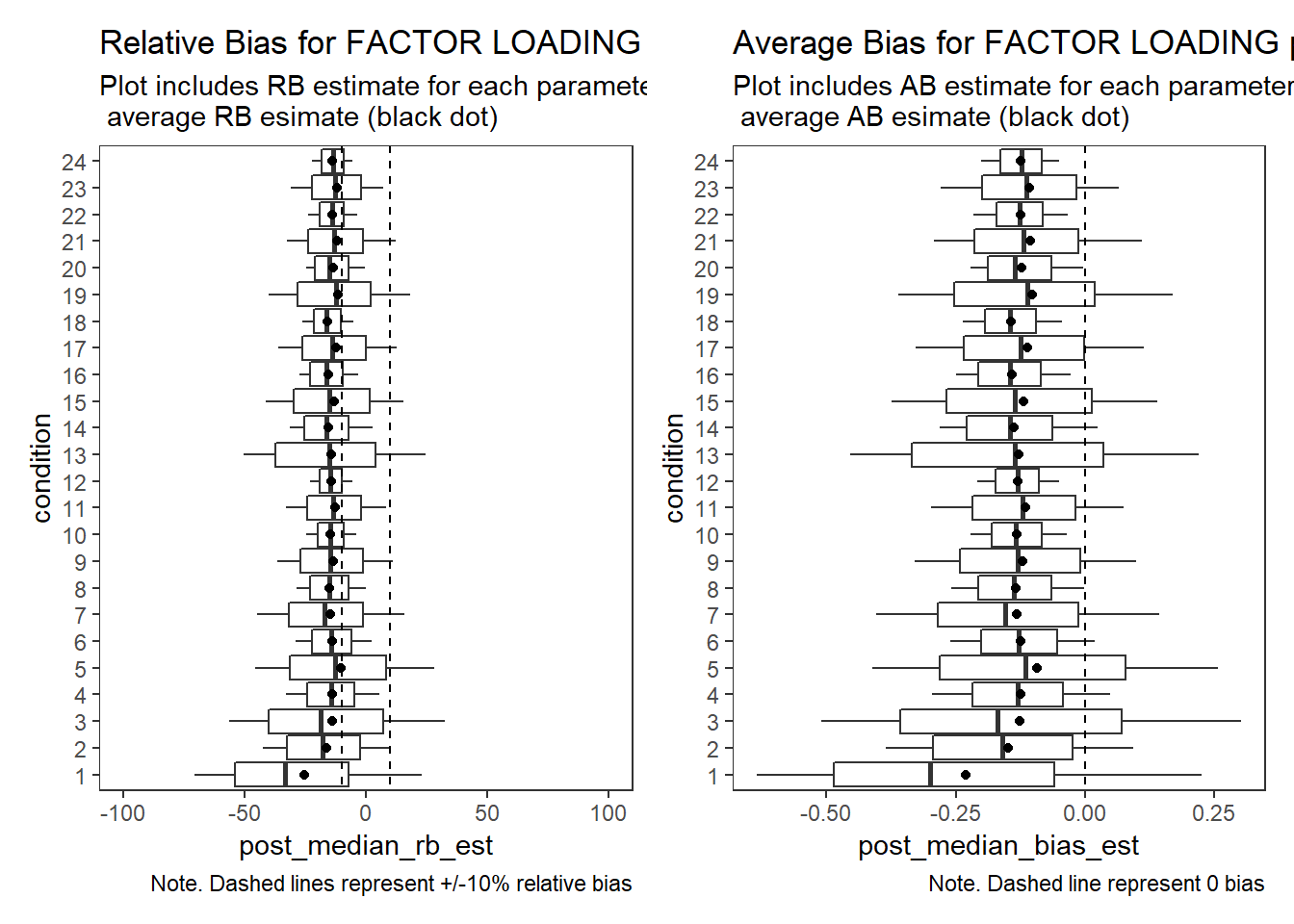
Item Thresholds (\(\tau\))
param = "Item Thresholds"

rb <- mydata %>%
  filter(parameter_group == "tau")

# tabular summary of relative bias
rb_tbl <- rb %>%
  group_by(condition, N_cat, N_items, N) %>%
  summarise(N_converge = n(),
            true = mean(true_value),
            avg_median_est = mean(post_q50),
            avg_mean_est = mean(post_mean),
            Post_Median_RB_Mean = mean(post_median_rb_est),
            Post_Median_RB_SD = sd(post_median_rb_est),
            Post_Mean_RB_Mean = mean(post_mean_rb_est),
            Post_Mean_RB_SD = sd(post_mean_rb_est),
            Post_Median_AB = mean(post_median_bias_est),
            Post_Mean_AB = mean(post_mean_bias_est))
`summarise()` has grouped output by 'condition', 'N_cat', 'N_items'. You can override using the `.groups` argument.kable(rb_tbl, format="html", digits=3) %>%
kable_styling(full_width = T) %>%
scroll_box(width="100%",height = "100%")| condition | N_cat | N_items | N | N_converge | true | avg_median_est | avg_mean_est | Post_Median_RB_Mean | Post_Median_RB_SD | Post_Mean_RB_Mean | Post_Mean_RB_SD | Post_Median_AB | Post_Mean_AB |
|---|---|---|---|---|---|---|---|---|---|---|---|---|---|
| 1 | 2 | 5 | 500 | 478 | 0.031 | 0.031 | 0.033 | -8.28 | 129.2 | -6.41 | 132.0 | 0.000 | 0.002 |
| 2 | 2 | 5 | 2500 | 491 | 0.032 | 0.029 | 0.029 | -2.28 | 56.4 | -1.66 | 56.7 | -0.003 | -0.002 |
| 3 | 2 | 10 | 500 | 985 | -0.046 | -0.041 | -0.041 | -2.85 | 112.5 | -1.55 | 114.1 | 0.005 | 0.005 |
| 4 | 2 | 10 | 2500 | 1000 | -0.046 | -0.050 | -0.050 | -3.30 | 46.6 | -3.16 | 46.7 | -0.004 | -0.004 |
| 5 | 2 | 20 | 500 | 2000 | -0.050 | -0.056 | -0.056 | 6.40 | 1480.3 | 8.90 | 1493.2 | -0.006 | -0.006 |
| 6 | 2 | 20 | 2500 | 2000 | -0.050 | -0.053 | -0.053 | -15.94 | 746.1 | -15.52 | 746.7 | -0.003 | -0.003 |
| 7 | 5 | 5 | 500 | 1943 | 0.299 | 0.301 | 0.303 | -3.81 | 46.7 | -3.19 | 47.1 | 0.002 | 0.004 |
| 8 | 5 | 5 | 2500 | 1997 | 0.303 | 0.284 | 0.284 | -8.11 | 19.6 | -8.03 | 19.7 | -0.019 | -0.019 |
| 9 | 5 | 10 | 500 | 3980 | 0.281 | 0.281 | 0.282 | -6.67 | 91.3 | -6.44 | 91.6 | 0.000 | 0.000 |
| 10 | 5 | 10 | 2500 | 3998 | 0.284 | 0.274 | 0.274 | -9.11 | 42.7 | -9.07 | 42.6 | -0.010 | -0.010 |
| 11 | 5 | 20 | 500 | 7970 | 0.278 | 0.290 | 0.291 | -22.63 | 433.6 | -22.57 | 433.9 | 0.012 | 0.013 |
| 12 | 5 | 20 | 2500 | 7990 | 0.279 | 0.269 | 0.269 | -16.54 | 170.1 | -16.53 | 170.3 | -0.010 | -0.010 |
| 13 | 3 | 5 | 500 | 977 | -0.288 | -0.165 | -0.167 | 58.04 | 115.6 | 59.29 | 116.4 | 0.123 | 0.121 |
| 14 | 3 | 5 | 2500 | 1000 | -0.292 | -0.172 | -0.173 | 54.39 | 96.7 | 54.54 | 96.8 | 0.120 | 0.119 |
| 15 | 3 | 10 | 500 | 1997 | -0.266 | -0.151 | -0.152 | -50.96 | 224.2 | -50.63 | 224.7 | 0.114 | 0.113 |
| 16 | 3 | 10 | 2500 | 2000 | -0.266 | -0.153 | -0.153 | -48.43 | 182.5 | -48.33 | 182.5 | 0.113 | 0.113 |
| 17 | 3 | 20 | 500 | 4000 | -0.293 | -0.184 | -0.184 | -67.29 | 672.9 | -66.92 | 673.2 | 0.109 | 0.108 |
| 18 | 3 | 20 | 2500 | 4000 | -0.293 | -0.185 | -0.185 | -52.74 | 443.1 | -52.69 | 443.1 | 0.108 | 0.108 |
| 19 | 7 | 5 | 500 | 2854 | 0.055 | 0.085 | 0.086 | -11.43 | 75.1 | -10.96 | 75.8 | 0.030 | 0.031 |
| 20 | 7 | 5 | 2500 | 1483 | 0.049 | 0.049 | 0.049 | -11.29 | 29.5 | -11.21 | 29.4 | 0.000 | 0.000 |
| 21 | 7 | 10 | 500 | 2971 | 0.045 | 0.073 | 0.074 | -6.00 | 95.5 | -5.74 | 95.8 | 0.028 | 0.028 |
| 22 | 7 | 10 | 2500 | 2989 | 0.044 | 0.054 | 0.054 | -8.05 | 47.1 | -8.01 | 47.2 | 0.010 | 0.010 |
| 23 | 7 | 20 | 500 | 5933 | 0.035 | 0.077 | 0.077 | 7.31 | 724.4 | 7.78 | 728.1 | 0.042 | 0.042 |
| 24 | 7 | 20 | 2500 | 4538 | 0.037 | 0.045 | 0.045 | -2.09 | 293.1 | -2.09 | 292.9 | 0.008 | 0.008 |
# visualize RB estimates
p1 <- ggplot() +
  stat_summary(
    data = rb,
    aes(x = condition, y = post_median_rb_est,
        group = condition),
    fun.data = cust.boxplot,
    geom = "boxplot"
  ) +
  geom_point(data = rb_tbl,
             aes(x = condition, y = Post_Median_RB_Mean),
             color = "black") +
  geom_abline(intercept = -10,
              slope = 0,
              linetype = "dashed") +
  geom_abline(intercept = 10,
              slope = 0,
              linetype = "dashed") +
  lims(y = c(-100, 100)) +
  coord_flip() +
  labs(
    title = paste0("Relative Bias for ", param, " posterior median"),
    subtitle = "Plot includes RB estimate for each parameter estimate (boxplot) and\n average RB esimate (black dot)",
    caption = "Note. Dashed lines represent +/-10% relative bias"
  ) +
  theme_bw() +
  theme(panel.grid = element_blank())
p2 <- ggplot() +
  stat_summary(
    data = rb,
    aes(x = condition, y = post_median_bias_est,
        group = condition),
    fun.data = cust.boxplot,
    geom = "boxplot"
  ) +
  geom_point(data = rb_tbl,
             aes(x = condition, y = Post_Median_AB),
             color = "black") +
  geom_abline(intercept = 0,
              slope = 0,
              linetype = "dashed")+
  coord_flip() +
  labs(
    title = paste0("Average Bias for ", param, " posterior median"),
    subtitle = "Plot includes AB estimate for each parameter estimate (boxplot) and\n average AB esimate (black dot)",
    caption = "Note. Dashed line represent 0 bias"
  ) +
  theme_bw() +
  theme(panel.grid = element_blank())
p1 + p2
Warning: Removed 7514 rows containing non-finite values (stat_summary).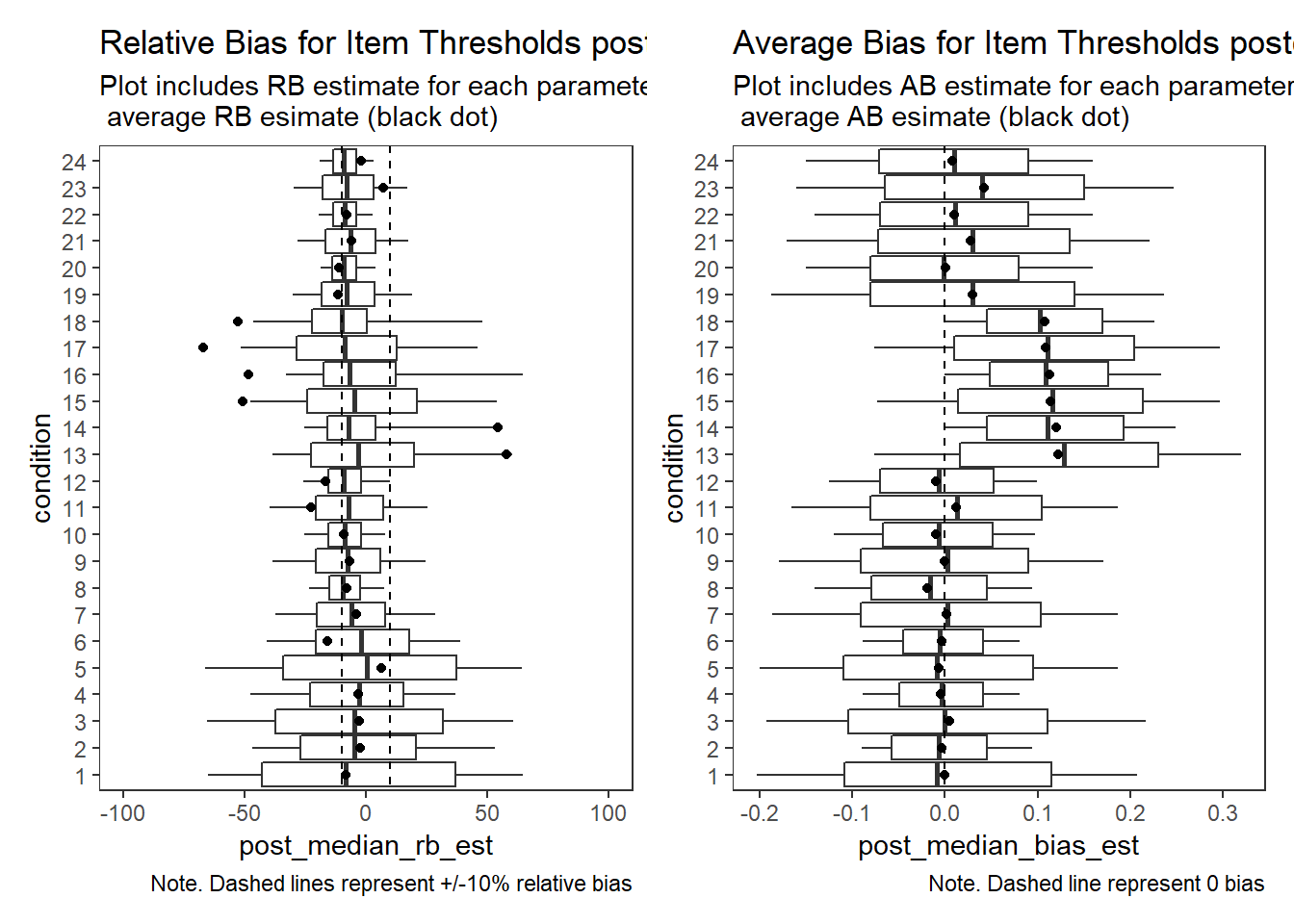
Latent Response Variance (\(\theta\))
param = "Latent Response Variance"

rb <- mydata %>%
  filter(parameter_group == "theta")

# tabular summary of relative bias
rb_tbl <- rb %>%
  group_by(condition, N_cat, N_items, N) %>%
  summarise(N_converge = n(),
            true = mean(true_value),
            avg_median_est = mean(post_q50),
            avg_mean_est = mean(post_mean),
            Post_Median_RB_Mean = mean(post_median_rb_est),
            Post_Median_RB_SD = sd(post_median_rb_est),
            Post_Mean_RB_Mean = mean(post_mean_rb_est),
            Post_Mean_RB_SD = sd(post_mean_rb_est),
            Post_Median_AB = mean(post_median_bias_est),
            Post_Mean_AB = mean(post_mean_bias_est))
`summarise()` has grouped output by 'condition', 'N_cat', 'N_items'. You can override using the `.groups` argument.kable(rb_tbl, format="html", digits=3) %>%
kable_styling(full_width = T) %>%
scroll_box(width="100%",height = "100%")| condition | N_cat | N_items | N | N_converge | true | avg_median_est | avg_mean_est | Post_Median_RB_Mean | Post_Median_RB_SD | Post_Mean_RB_Mean | Post_Mean_RB_SD | Post_Median_AB | Post_Mean_AB |
|---|---|---|---|---|---|---|---|---|---|---|---|---|---|
| 1 | 2 | 5 | 500 | 250 | 1.81 | 1.63 | 1.87 | -9.86 | 37.55 | 3.127 | 46.48 | -0.179 | 0.057 |
| 2 | 2 | 5 | 2500 | 310 | 1.81 | 1.60 | 1.66 | -11.40 | 16.23 | -8.439 | 17.21 | -0.206 | -0.153 |
| 3 | 2 | 10 | 500 | 756 | 1.81 | 1.71 | 1.88 | -5.68 | 32.22 | 3.674 | 37.81 | -0.103 | 0.066 |
| 4 | 2 | 10 | 2500 | 887 | 1.81 | 1.62 | 1.65 | -10.66 | 11.96 | -9.057 | 12.37 | -0.193 | -0.164 |
| 5 | 2 | 20 | 500 | 1844 | 1.81 | 1.72 | 1.83 | -4.72 | 26.70 | 1.397 | 29.74 | -0.086 | 0.025 |
| 6 | 2 | 20 | 2500 | 1941 | 1.81 | 1.61 | 1.63 | -10.85 | 9.46 | -9.902 | 9.64 | -0.196 | -0.179 |
| 7 | 5 | 5 | 500 | 366 | 1.81 | 1.64 | 1.73 | -9.39 | 21.81 | -4.619 | 25.77 | -0.170 | -0.084 |
| 8 | 5 | 5 | 2500 | 452 | 1.81 | 1.60 | 1.61 | -11.81 | 8.47 | -11.042 | 8.61 | -0.214 | -0.200 |
| 9 | 5 | 10 | 500 | 908 | 1.81 | 1.63 | 1.67 | -9.83 | 15.24 | -7.650 | 15.98 | -0.178 | -0.138 |
| 10 | 5 | 10 | 2500 | 964 | 1.81 | 1.60 | 1.60 | -11.84 | 6.23 | -11.435 | 6.28 | -0.214 | -0.207 |
| 11 | 5 | 20 | 500 | 1876 | 1.81 | 1.64 | 1.66 | -9.50 | 13.20 | -8.019 | 13.56 | -0.172 | -0.145 |
| 12 | 5 | 20 | 2500 | 1932 | 1.81 | 1.60 | 1.60 | -11.76 | 5.25 | -11.498 | 5.28 | -0.213 | -0.208 |
| 13 | 3 | 5 | 500 | 402 | 1.81 | 1.68 | 1.80 | -7.28 | 26.35 | -0.301 | 30.88 | -0.132 | -0.005 |
| 14 | 3 | 5 | 2500 | 465 | 1.81 | 1.59 | 1.62 | -11.89 | 10.86 | -10.744 | 11.23 | -0.215 | -0.194 |
| 15 | 3 | 10 | 500 | 976 | 1.81 | 1.65 | 1.72 | -8.71 | 20.05 | -5.268 | 21.45 | -0.158 | -0.095 |
| 16 | 3 | 10 | 2500 | 993 | 1.81 | 1.58 | 1.59 | -12.49 | 7.65 | -11.918 | 7.76 | -0.226 | -0.216 |
| 17 | 3 | 20 | 500 | 1986 | 1.81 | 1.65 | 1.69 | -8.87 | 15.77 | -6.593 | 16.50 | -0.161 | -0.119 |
| 18 | 3 | 20 | 2500 | 2000 | 1.81 | 1.58 | 1.59 | -12.77 | 6.29 | -12.384 | 6.34 | -0.231 | -0.224 |
| 19 | 7 | 5 | 500 | 374 | 1.81 | 1.68 | 1.75 | -7.13 | 21.88 | -3.121 | 24.43 | -0.129 | -0.056 |
| 20 | 7 | 5 | 2500 | 205 | 1.81 | 1.61 | 1.62 | -11.17 | 7.52 | -10.543 | 7.62 | -0.202 | -0.191 |
| 21 | 7 | 10 | 500 | 420 | 1.81 | 1.65 | 1.69 | -8.71 | 13.99 | -6.860 | 14.50 | -0.158 | -0.124 |
| 22 | 7 | 10 | 2500 | 451 | 1.81 | 1.61 | 1.61 | -11.27 | 5.98 | -10.919 | 6.03 | -0.204 | -0.198 |
| 23 | 7 | 20 | 500 | 861 | 1.81 | 1.65 | 1.67 | -8.93 | 12.52 | -7.658 | 12.80 | -0.162 | -0.139 |
| 24 | 7 | 20 | 2500 | 700 | 1.81 | 1.61 | 1.61 | -11.28 | 5.04 | -11.037 | 5.06 | -0.204 | -0.200 |
# visualize RB estimates
p1 <- ggplot() +
  stat_summary(
    data = rb,
    aes(x = condition, y = post_median_rb_est,
        group = condition),
    fun.data = cust.boxplot,
    geom = "boxplot"
  ) +
  geom_point(data = rb_tbl,
             aes(x = condition, y = Post_Median_RB_Mean),
             color = "black") +
  geom_abline(intercept = -10,
              slope = 0,
              linetype = "dashed") +
  geom_abline(intercept = 10,
              slope = 0,
              linetype = "dashed") +
  lims(y = c(-100, 100)) +
  coord_flip() +
  labs(
    title = paste0("Relative Bias for ", param, " posterior median"),
    subtitle = "Plot includes RB estimate for each parameter estimate (boxplot) and\n average RB esimate (black dot)",
    caption = "Note. Dashed lines represent +/-10% relative bias"
  ) +
  theme_bw() +
  theme(panel.grid = element_blank())
p2 <- ggplot() +
  stat_summary(
    data = rb,
    aes(x = condition, y = post_median_bias_est,
        group = condition),
    fun.data = cust.boxplot,
    geom = "boxplot"
  ) +
  geom_point(data = rb_tbl,
             aes(x = condition, y = Post_Median_AB),
             color = "black") +
  geom_abline(intercept = 0,
              slope = 0,
              linetype = "dashed")+
  coord_flip() +
  labs(
    title = paste0("Average Bias for ", param, " posterior median"),
    subtitle = "Plot includes AB estimate for each parameter estimate (boxplot) and\n average AB esimate (black dot)",
    caption = "Note. Dashed line represent 0 bias"
  ) +
  theme_bw() +
  theme(panel.grid = element_blank())
p1 + p2
Warning: Removed 31 rows containing non-finite values (stat_summary).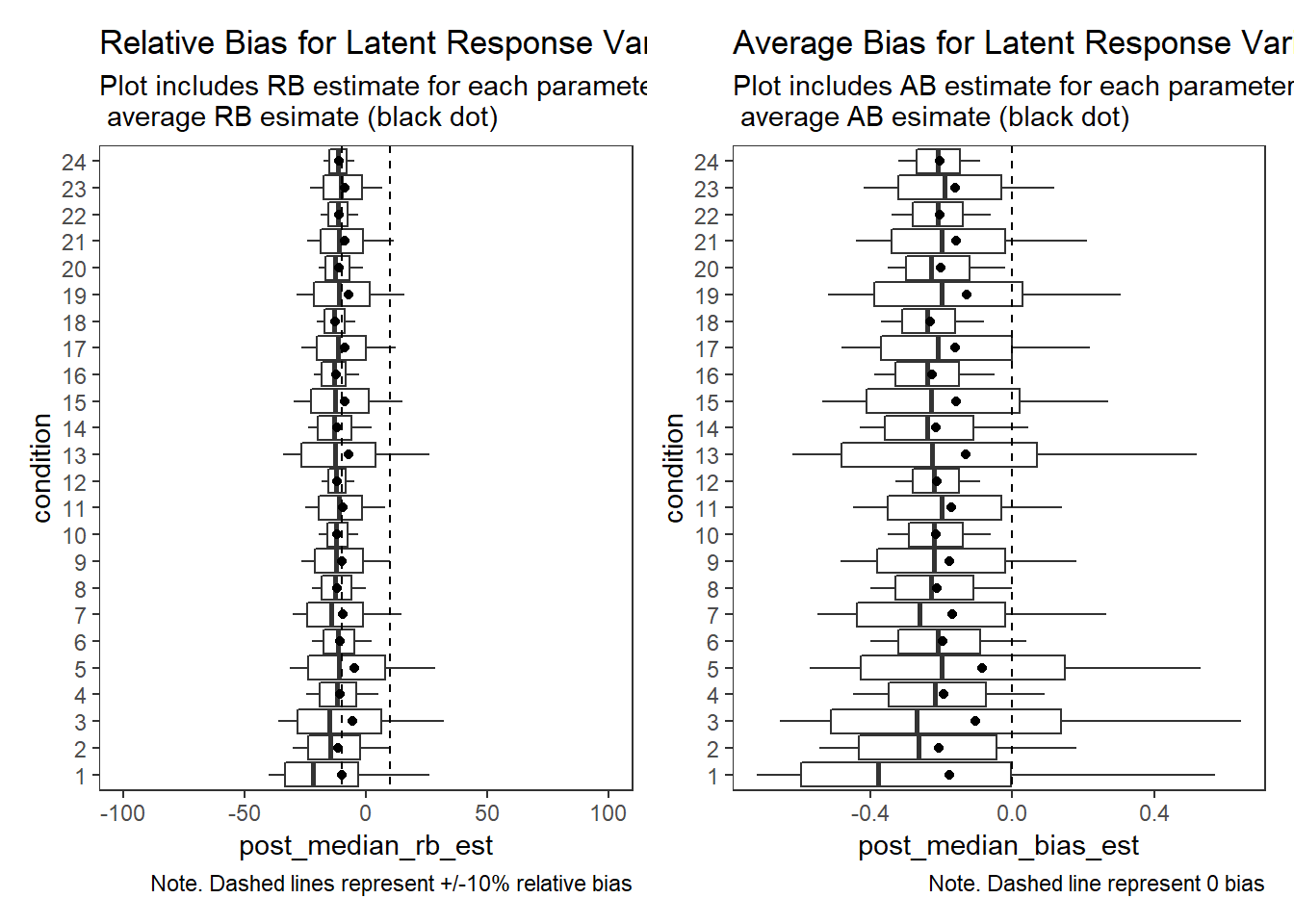
Response Time Intercepts (\(\beta_{lrt}\))
param = "RT Intercepts"

rb <- mydata %>%
  filter(parameter_group == "beta_lrt")

# tabular summary of relative bias
rb_tbl <- rb %>%
  group_by(condition, N_cat, N_items, N) %>%
  summarise(N_converge = n(),
            true = mean(true_value),
            avg_median_est = mean(post_q50),
            avg_mean_est = mean(post_mean),
            Post_Median_RB_Mean = mean(post_median_rb_est),
            Post_Median_RB_SD = sd(post_median_rb_est),
            Post_Mean_RB_Mean = mean(post_mean_rb_est),
            Post_Mean_RB_SD = sd(post_mean_rb_est),
            Post_Median_AB = mean(post_median_bias_est),
            Post_Mean_AB = mean(post_mean_bias_est))
`summarise()` has grouped output by 'condition', 'N_cat', 'N_items'. You can override using the `.groups` argument.kable(rb_tbl, format="html", digits=3) %>%
kable_styling(full_width = T) %>%
scroll_box(width="100%",height = "100%")| condition | N_cat | N_items | N | N_converge | true | avg_median_est | avg_mean_est | Post_Median_RB_Mean | Post_Median_RB_SD | Post_Mean_RB_Mean | Post_Mean_RB_SD | Post_Median_AB | Post_Mean_AB |
|---|---|---|---|---|---|---|---|---|---|---|---|---|---|
| 1 | 2 | 5 | 500 | 402 | 1.5 | 1.50 | 1.51 | 0.091 | 4.01 | 0.618 | 3.91 | 0.001 | 0.009 |
| 2 | 2 | 5 | 2500 | 401 | 1.5 | 1.51 | 1.51 | 0.547 | 2.53 | 0.694 | 2.49 | 0.008 | 0.010 |
| 3 | 2 | 10 | 500 | 927 | 1.5 | 1.48 | 1.49 | -1.067 | 3.09 | -0.817 | 3.10 | -0.016 | -0.012 |
| 4 | 2 | 10 | 2500 | 974 | 1.5 | 1.51 | 1.51 | 0.559 | 1.75 | 0.630 | 1.74 | 0.008 | 0.009 |
| 5 | 2 | 20 | 500 | 1986 | 1.5 | 1.48 | 1.48 | -1.312 | 2.46 | -1.194 | 2.47 | -0.020 | -0.018 |
| 6 | 2 | 20 | 2500 | 1999 | 1.5 | 1.50 | 1.50 | 0.299 | 1.32 | 0.332 | 1.32 | 0.004 | 0.005 |
| 7 | 5 | 5 | 500 | 464 | 1.5 | 1.51 | 1.51 | 0.533 | 3.69 | 0.805 | 3.63 | 0.008 | 0.012 |
| 8 | 5 | 5 | 2500 | 488 | 1.5 | 1.52 | 1.52 | 1.423 | 2.09 | 1.467 | 2.09 | 0.021 | 0.022 |
| 9 | 5 | 10 | 500 | 984 | 1.5 | 1.50 | 1.50 | -0.303 | 2.76 | -0.199 | 2.75 | -0.005 | -0.003 |
| 10 | 5 | 10 | 2500 | 1000 | 1.5 | 1.51 | 1.51 | 0.569 | 1.33 | 0.595 | 1.33 | 0.009 | 0.009 |
| 11 | 5 | 20 | 500 | 1995 | 1.5 | 1.49 | 1.49 | -0.819 | 2.62 | -0.771 | 2.62 | -0.012 | -0.012 |
| 12 | 5 | 20 | 2500 | 2000 | 1.5 | 1.51 | 1.51 | 0.389 | 1.09 | 0.401 | 1.09 | 0.006 | 0.006 |
| 13 | 3 | 5 | 500 | 480 | 1.5 | 1.50 | 1.51 | 0.353 | 3.97 | 0.692 | 3.90 | 0.005 | 0.010 |
| 14 | 3 | 5 | 2500 | 494 | 1.5 | 1.52 | 1.52 | 1.428 | 2.21 | 1.513 | 2.20 | 0.021 | 0.023 |
| 15 | 3 | 10 | 500 | 996 | 1.5 | 1.50 | 1.50 | 0.051 | 3.06 | 0.205 | 3.05 | 0.001 | 0.003 |
| 16 | 3 | 10 | 2500 | 1000 | 1.5 | 1.51 | 1.51 | 0.753 | 1.53 | 0.789 | 1.52 | 0.011 | 0.012 |
| 17 | 3 | 20 | 500 | 2000 | 1.5 | 1.49 | 1.49 | -0.779 | 2.40 | -0.716 | 2.40 | -0.012 | -0.011 |
| 18 | 3 | 20 | 2500 | 2000 | 1.5 | 1.50 | 1.50 | 0.064 | 1.23 | 0.085 | 1.23 | 0.001 | 0.001 |
| 19 | 7 | 5 | 500 | 482 | 1.5 | 1.50 | 1.51 | 0.281 | 3.37 | 0.520 | 3.35 | 0.004 | 0.008 |
| 20 | 7 | 5 | 2500 | 237 | 1.5 | 1.52 | 1.52 | 1.226 | 1.72 | 1.246 | 1.72 | 0.018 | 0.019 |
| 21 | 7 | 10 | 500 | 497 | 1.5 | 1.50 | 1.50 | -0.144 | 2.49 | -0.054 | 2.49 | -0.002 | -0.001 |
| 22 | 7 | 10 | 2500 | 497 | 1.5 | 1.51 | 1.51 | 0.447 | 1.25 | 0.471 | 1.25 | 0.007 | 0.007 |
| 23 | 7 | 20 | 500 | 999 | 1.5 | 1.49 | 1.49 | -0.799 | 2.24 | -0.755 | 2.23 | -0.012 | -0.011 |
| 24 | 7 | 20 | 2500 | 760 | 1.5 | 1.50 | 1.50 | 0.172 | 1.07 | 0.180 | 1.07 | 0.003 | 0.003 |
# visualize RB estimates
p1 <- ggplot() +
  stat_summary(
    data = rb,
    aes(x = condition, y = post_median_rb_est,
        group = condition),
    fun.data = cust.boxplot,
    geom = "boxplot"
  ) +
  geom_point(data = rb_tbl,
             aes(x = condition, y = Post_Median_RB_Mean),
             color = "black") +
  geom_abline(intercept = -10,
              slope = 0,
              linetype = "dashed") +
  geom_abline(intercept = 10,
              slope = 0,
              linetype = "dashed") +
  lims(y = c(-100, 100)) +
  coord_flip() +
  labs(
    title = paste0("Relative Bias for ", param, " posterior median"),
    subtitle = "Plot includes RB estimate for each parameter estimate (boxplot) and\n average RB esimate (black dot)",
    caption = "Note. Dashed lines represent +/-10% relative bias"
  ) +
  theme_bw() +
  theme(panel.grid = element_blank())
p2 <- ggplot() +
  stat_summary(
    data = rb,
    aes(x = condition, y = post_median_bias_est,
        group = condition),
    fun.data = cust.boxplot,
    geom = "boxplot"
  ) +
  geom_point(data = rb_tbl,
             aes(x = condition, y = Post_Median_AB),
             color = "black") +
  geom_abline(intercept = 0,
              slope = 0,
              linetype = "dashed")+
  coord_flip() +
  labs(
    title = paste0("Average Bias for ", param, " posterior median"),
    subtitle = "Plot includes AB estimate for each parameter estimate (boxplot) and\n average AB esimate (black dot)",
    caption = "Note. Dashed line represent 0 bias"
  ) +
  theme_bw() +
  theme(panel.grid = element_blank())
p1 + p2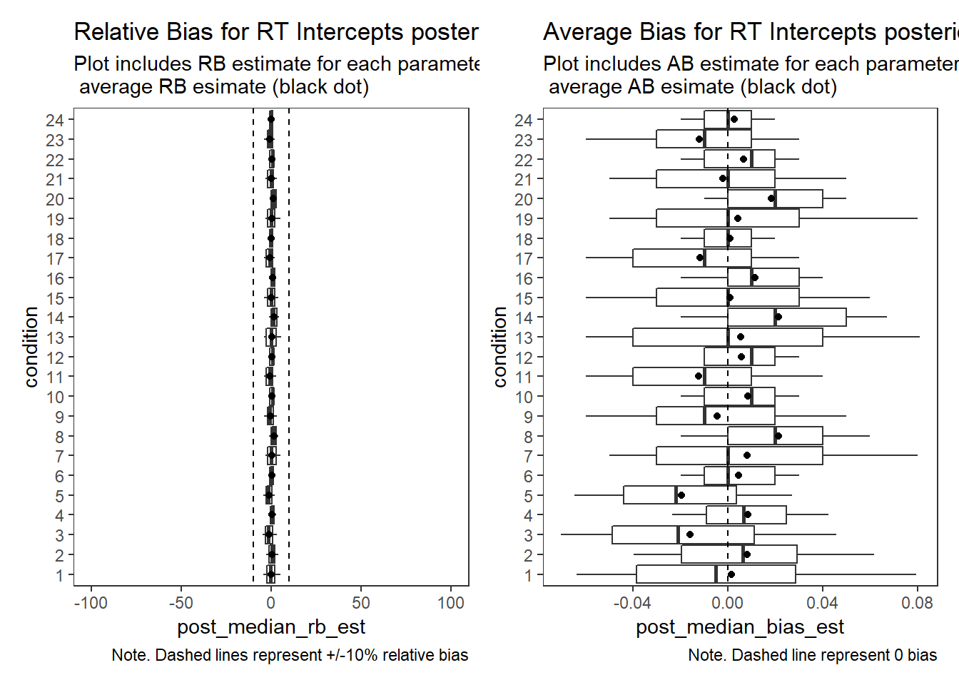
Response Time Precision (\(\sigma_{lrt}\))
param = "RT Precision"

rb <- mydata %>%
  filter(parameter_group == "sigma_lrt")

# tabular summary of relative bias
rb_tbl <- rb %>%
  group_by(condition, N_cat, N_items, N) %>%
  summarise(N_converge = n(),
            true = mean(true_value),
            avg_median_est = mean(post_q50),
            avg_mean_est = mean(post_mean),
            Post_Median_RB_Mean = mean(post_median_rb_est),
            Post_Median_RB_SD = sd(post_median_rb_est),
            Post_Mean_RB_Mean = mean(post_mean_rb_est),
            Post_Mean_RB_SD = sd(post_mean_rb_est),
            Post_Median_AB = mean(post_median_bias_est),
            Post_Mean_AB = mean(post_mean_bias_est))
`summarise()` has grouped output by 'condition', 'N_cat', 'N_items'. You can override using the `.groups` argument.kable(rb_tbl, format="html", digits=3) %>%
kable_styling(full_width = T) %>%
scroll_box(width="100%",height = "100%")| condition | N_cat | N_items | N | N_converge | true | avg_median_est | avg_mean_est | Post_Median_RB_Mean | Post_Median_RB_SD | Post_Mean_RB_Mean | Post_Mean_RB_SD | Post_Median_AB | Post_Mean_AB |
|---|---|---|---|---|---|---|---|---|---|---|---|---|---|
| 1 | 2 | 5 | 500 | 485 | 4 | 4.05 | 4.07 | 1.293 | 8.14 | 1.861 | 8.46 | 0.052 | 0.074 |
| 2 | 2 | 5 | 2500 | 497 | 4 | 4.02 | 4.02 | 0.417 | 3.30 | 0.495 | 3.31 | 0.017 | 0.020 |
| 3 | 2 | 10 | 500 | 998 | 4 | 4.03 | 4.04 | 0.660 | 7.00 | 0.889 | 7.03 | 0.026 | 0.036 |
| 4 | 2 | 10 | 2500 | 1000 | 4 | 4.01 | 4.01 | 0.139 | 3.21 | 0.180 | 3.21 | 0.006 | 0.007 |
| 5 | 2 | 20 | 500 | 2000 | 4 | 4.01 | 4.01 | 0.175 | 6.75 | 0.343 | 6.76 | 0.007 | 0.014 |
| 6 | 2 | 20 | 2500 | 2000 | 4 | 4.00 | 4.00 | 0.081 | 3.07 | 0.111 | 3.07 | 0.003 | 0.004 |
| 7 | 5 | 5 | 500 | 500 | 4 | 4.04 | 4.05 | 0.999 | 7.18 | 1.290 | 7.23 | 0.040 | 0.052 |
| 8 | 5 | 5 | 2500 | 500 | 4 | 4.01 | 4.01 | 0.153 | 3.45 | 0.206 | 3.45 | 0.006 | 0.008 |
| 9 | 5 | 10 | 500 | 1000 | 4 | 4.01 | 4.02 | 0.328 | 7.35 | 0.517 | 7.37 | 0.013 | 0.021 |
| 10 | 5 | 10 | 2500 | 1000 | 4 | 4.00 | 4.00 | 0.076 | 3.13 | 0.116 | 3.13 | 0.003 | 0.005 |
| 11 | 5 | 20 | 500 | 2000 | 4 | 4.01 | 4.02 | 0.312 | 6.60 | 0.468 | 6.61 | 0.012 | 0.019 |
| 12 | 5 | 20 | 2500 | 2000 | 4 | 4.00 | 4.01 | 0.132 | 2.93 | 0.165 | 2.93 | 0.005 | 0.007 |
| 13 | 3 | 5 | 500 | 499 | 4 | 4.04 | 4.05 | 0.962 | 7.19 | 1.309 | 7.28 | 0.038 | 0.052 |
| 14 | 3 | 5 | 2500 | 500 | 4 | 4.02 | 4.02 | 0.507 | 3.46 | 0.565 | 3.46 | 0.020 | 0.023 |
| 15 | 3 | 10 | 500 | 1000 | 4 | 4.01 | 4.02 | 0.268 | 6.74 | 0.463 | 6.76 | 0.011 | 0.019 |
| 16 | 3 | 10 | 2500 | 1000 | 4 | 4.01 | 4.01 | 0.211 | 3.08 | 0.246 | 3.08 | 0.008 | 0.010 |
| 17 | 3 | 20 | 500 | 2000 | 4 | 4.00 | 4.01 | 0.081 | 6.82 | 0.242 | 6.84 | 0.003 | 0.010 |
| 18 | 3 | 20 | 2500 | 2000 | 4 | 4.00 | 4.01 | 0.119 | 2.93 | 0.152 | 2.93 | 0.005 | 0.006 |
| 19 | 7 | 5 | 500 | 500 | 4 | 4.00 | 4.01 | -0.042 | 7.56 | 0.225 | 7.59 | -0.002 | 0.009 |
| 20 | 7 | 5 | 2500 | 250 | 4 | 4.00 | 4.00 | 0.036 | 3.24 | 0.090 | 3.24 | 0.001 | 0.004 |
| 21 | 7 | 10 | 500 | 500 | 4 | 4.01 | 4.02 | 0.247 | 6.94 | 0.435 | 6.95 | 0.010 | 0.017 |
| 22 | 7 | 10 | 2500 | 500 | 4 | 4.00 | 4.00 | 0.092 | 3.13 | 0.136 | 3.12 | 0.004 | 0.005 |
| 23 | 7 | 20 | 500 | 1000 | 4 | 4.00 | 4.00 | -0.031 | 6.52 | 0.128 | 6.53 | -0.001 | 0.005 |
| 24 | 7 | 20 | 2500 | 760 | 4 | 4.00 | 4.00 | 0.037 | 3.13 | 0.065 | 3.13 | 0.001 | 0.003 |
# visualize RB estimates
p1 <- ggplot() +
  stat_summary(
    data = rb,
    aes(x = condition, y = post_median_rb_est,
        group = condition),
    fun.data = cust.boxplot,
    geom = "boxplot"
  ) +
  geom_point(data = rb_tbl,
             aes(x = condition, y = Post_Median_RB_Mean),
             color = "black") +
  geom_abline(intercept = -10,
              slope = 0,
              linetype = "dashed") +
  geom_abline(intercept = 10,
              slope = 0,
              linetype = "dashed") +
  lims(y = c(-100, 100)) +
  coord_flip() +
  labs(
    title = paste0("Relative Bias for ", param, " posterior median"),
    subtitle = "Plot includes RB estimate for each parameter estimate (boxplot) and\n average RB esimate (black dot)",
    caption = "Note. Dashed lines represent +/-10% relative bias"
  ) +
  theme_bw() +
  theme(panel.grid = element_blank())
p2 <- ggplot() +
  stat_summary(
    data = rb,
    aes(x = condition, y = post_median_bias_est,
        group = condition),
    fun.data = cust.boxplot,
    geom = "boxplot"
  ) +
  geom_point(data = rb_tbl,
             aes(x = condition, y = Post_Median_AB),
             color = "black") +
  geom_abline(intercept = 0,
              slope = 0,
              linetype = "dashed")+
  coord_flip() +
  labs(
    title = paste0("Average Bias for ", param, " posterior median"),
    subtitle = "Plot includes AB estimate for each parameter estimate (boxplot) and\n average AB esimate (black dot)",
    caption = "Note. Dashed line represent 0 bias"
  ) +
  theme_bw() +
  theme(panel.grid = element_blank())
p1 + p2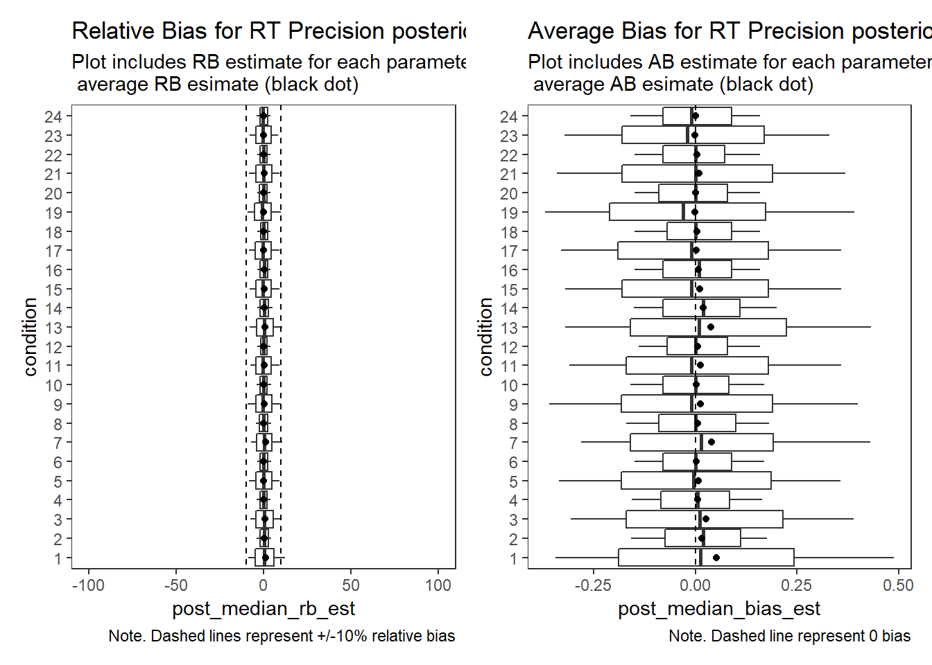
Response Time Factor Precision (\(\sigma_s\))
param = "Speed LV Precision"

rb <- mydata %>%
  filter(parameter_group == "sigma_s")

# tabular summary of relative bias
rb_tbl <- rb %>%
  group_by(condition, N_cat, N_items, N) %>%
  summarise(N_converge = n(),
            true = mean(true_value),
            avg_median_est = mean(post_q50),
            avg_mean_est = mean(post_mean),
            Post_Median_RB_Mean = mean(post_median_rb_est),
            Post_Median_RB_SD = sd(post_median_rb_est),
            Post_Mean_RB_Mean = mean(post_mean_rb_est),
            Post_Mean_RB_SD = sd(post_mean_rb_est),
            Post_Median_AB = mean(post_median_bias_est),
            Post_Mean_AB = mean(post_mean_bias_est))
`summarise()` has grouped output by 'condition', 'N_cat', 'N_items'. You can override using the `.groups` argument.kable(rb_tbl, format="html", digits=3) %>%
kable_styling(full_width = T) %>%
scroll_box(width="100%",height = "100%")| condition | N_cat | N_items | N | N_converge | true | avg_median_est | avg_mean_est | Post_Median_RB_Mean | Post_Median_RB_SD | Post_Mean_RB_Mean | Post_Mean_RB_SD | Post_Median_AB | Post_Mean_AB |
|---|---|---|---|---|---|---|---|---|---|---|---|---|---|
| 1 | 2 | 5 | 500 | 99 | 10 | 11.2 | 11.4 | 11.63 | 13.96 | 13.88 | 14.87 | 1.164 | 1.388 |
| 2 | 2 | 5 | 2500 | 97 | 10 | 10.8 | 10.8 | 7.68 | 6.82 | 8.10 | 6.91 | 0.768 | 0.810 |
| 3 | 2 | 10 | 500 | 100 | 10 | 10.6 | 10.7 | 6.25 | 9.73 | 6.86 | 9.91 | 0.625 | 0.686 |
| 4 | 2 | 10 | 2500 | 100 | 10 | 10.7 | 10.7 | 6.77 | 4.41 | 6.92 | 4.42 | 0.677 | 0.693 |
| 5 | 2 | 20 | 500 | 100 | 10 | 10.4 | 10.5 | 4.35 | 9.11 | 4.67 | 9.15 | 0.435 | 0.467 |
| 6 | 2 | 20 | 2500 | 100 | 10 | 10.6 | 10.6 | 5.76 | 3.65 | 5.83 | 3.63 | 0.576 | 0.583 |
| 7 | 5 | 5 | 500 | 100 | 10 | 11.0 | 11.1 | 10.07 | 12.04 | 11.18 | 12.37 | 1.007 | 1.118 |
| 8 | 5 | 5 | 2500 | 100 | 10 | 10.8 | 10.8 | 8.09 | 5.87 | 8.34 | 5.87 | 0.809 | 0.834 |
| 9 | 5 | 10 | 500 | 100 | 10 | 10.7 | 10.8 | 7.25 | 8.18 | 7.71 | 8.23 | 0.725 | 0.771 |
| 10 | 5 | 10 | 2500 | 100 | 10 | 10.7 | 10.7 | 6.86 | 4.12 | 6.95 | 4.15 | 0.686 | 0.695 |
| 11 | 5 | 20 | 500 | 100 | 10 | 10.6 | 10.6 | 6.22 | 7.36 | 6.46 | 7.38 | 0.622 | 0.646 |
| 12 | 5 | 20 | 2500 | 100 | 10 | 10.6 | 10.6 | 5.71 | 2.94 | 5.79 | 2.97 | 0.572 | 0.580 |
| 13 | 3 | 5 | 500 | 100 | 10 | 10.8 | 11.0 | 8.40 | 12.55 | 9.91 | 13.22 | 0.840 | 0.991 |
| 14 | 3 | 5 | 2500 | 100 | 10 | 10.9 | 10.9 | 8.63 | 6.00 | 9.15 | 6.11 | 0.863 | 0.915 |
| 15 | 3 | 10 | 500 | 100 | 10 | 10.7 | 10.7 | 6.76 | 9.38 | 7.31 | 9.51 | 0.676 | 0.731 |
| 16 | 3 | 10 | 2500 | 100 | 10 | 10.8 | 10.8 | 8.05 | 4.77 | 8.17 | 4.74 | 0.805 | 0.817 |
| 17 | 3 | 20 | 500 | 100 | 10 | 10.6 | 10.6 | 6.08 | 7.88 | 6.42 | 7.91 | 0.608 | 0.642 |
| 18 | 3 | 20 | 2500 | 100 | 10 | 10.6 | 10.6 | 6.18 | 3.48 | 6.24 | 3.46 | 0.618 | 0.624 |
| 19 | 7 | 5 | 500 | 100 | 10 | 10.9 | 11.0 | 8.80 | 10.85 | 9.89 | 11.26 | 0.880 | 0.989 |
| 20 | 7 | 5 | 2500 | 50 | 10 | 10.8 | 10.8 | 8.05 | 4.92 | 8.26 | 5.07 | 0.805 | 0.826 |
| 21 | 7 | 10 | 500 | 50 | 10 | 10.5 | 10.6 | 5.45 | 9.35 | 5.93 | 9.48 | 0.545 | 0.593 |
| 22 | 7 | 10 | 2500 | 50 | 10 | 10.6 | 10.6 | 6.34 | 3.62 | 6.44 | 3.68 | 0.634 | 0.644 |
| 23 | 7 | 20 | 500 | 50 | 10 | 10.8 | 10.8 | 7.58 | 7.40 | 7.88 | 7.46 | 0.758 | 0.788 |
| 24 | 7 | 20 | 2500 | 38 | 10 | 10.6 | 10.6 | 5.89 | 3.39 | 5.97 | 3.42 | 0.589 | 0.597 |
# visualize RB estimates
p1 <- ggplot() +
  stat_summary(
    data = rb,
    aes(x = condition, y = post_median_rb_est,
        group = condition),
    fun.data = cust.boxplot,
    geom = "boxplot"
  ) +
  geom_point(data = rb_tbl,
             aes(x = condition, y = Post_Median_RB_Mean),
             color = "black") +
  geom_abline(intercept = -10,
              slope = 0,
              linetype = "dashed") +
  geom_abline(intercept = 10,
              slope = 0,
              linetype = "dashed") +
  lims(y = c(-100, 100)) +
  coord_flip() +
  labs(
    title = paste0("Relative Bias for ", param, " posterior median"),
    subtitle = "Plot includes RB estimate for each parameter estimate (boxplot) and\n average RB esimate (black dot)",
    caption = "Note. Dashed lines represent +/-10% relative bias"
  ) +
  theme_bw() +
  theme(panel.grid = element_blank())
p2 <- ggplot() +
  stat_summary(
    data = rb,
    aes(x = condition, y = post_median_bias_est,
        group = condition),
    fun.data = cust.boxplot,
    geom = "boxplot"
  ) +
  geom_point(data = rb_tbl,
             aes(x = condition, y = Post_Median_AB),
             color = "black") +
  geom_abline(intercept = 0,
              slope = 0,
              linetype = "dashed")+
  coord_flip() +
  labs(
    title = paste0("Average Bias for ", param, " posterior median"),
    subtitle = "Plot includes AB estimate for each parameter estimate (boxplot) and\n average AB esimate (black dot)",
    caption = "Note. Dashed line represent 0 bias"
  ) +
  theme_bw() +
  theme(panel.grid = element_blank())
p1 + p2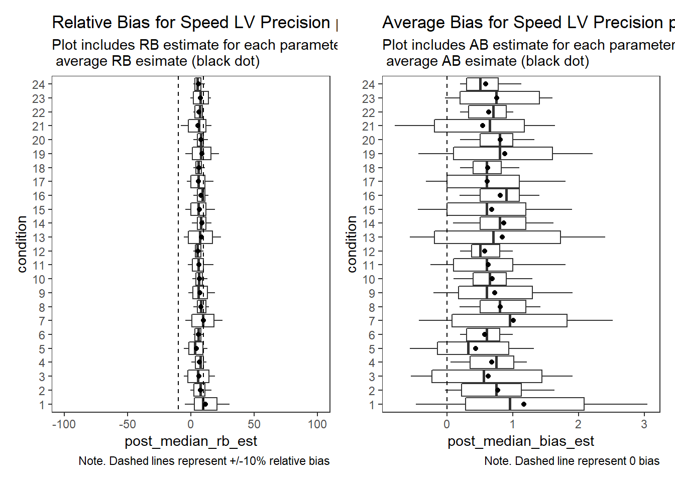
Factor Covariance (\(\sigma_{st}\))
param = "Latent Covariance"

rb <- mydata %>%
  filter(parameter_group == "sigma_st")

# tabular summary of relative bias
rb_tbl <- rb %>%
  group_by(condition, N_cat, N_items, N) %>%
  summarise(N_converge = n(),
            true = mean(true_value),
            avg_median_est = mean(post_q50),
            avg_mean_est = mean(post_mean),
            Post_Median_RB_Mean = mean(post_median_rb_est),
            Post_Median_RB_SD = sd(post_median_rb_est),
            Post_Mean_RB_Mean = mean(post_mean_rb_est),
            Post_Mean_RB_SD = sd(post_mean_rb_est),
            Post_Median_AB = mean(post_median_bias_est),
            Post_Mean_AB = mean(post_mean_bias_est))
`summarise()` has grouped output by 'condition', 'N_cat', 'N_items'. You can override using the `.groups` argument.kable(rb_tbl, format="html", digits=3) %>%
kable_styling(full_width = T) %>%
scroll_box(width="100%",height = "100%")| condition | N_cat | N_items | N | N_converge | true | avg_median_est | avg_mean_est | Post_Median_RB_Mean | Post_Median_RB_SD | Post_Mean_RB_Mean | Post_Mean_RB_SD | Post_Median_AB | Post_Mean_AB |
|---|---|---|---|---|---|---|---|---|---|---|---|---|---|
| 1 | 2 | 5 | 500 | 95 | -0.073 | -0.066 | -0.065 | -9.696 | 53.0 | -10.159 | 52.7 | 0.007 | 0.007 |
| 2 | 2 | 5 | 2500 | 98 | -0.073 | -0.067 | -0.067 | -7.757 | 24.1 | -7.722 | 24.1 | 0.006 | 0.006 |
| 3 | 2 | 10 | 500 | 100 | -0.073 | -0.068 | -0.068 | -6.543 | 40.5 | -6.705 | 40.4 | 0.005 | 0.005 |
| 4 | 2 | 10 | 2500 | 100 | -0.073 | -0.071 | -0.071 | -2.674 | 15.7 | -2.682 | 15.6 | 0.002 | 0.002 |
| 5 | 2 | 20 | 500 | 100 | -0.073 | -0.070 | -0.070 | -4.398 | 29.1 | -4.436 | 29.0 | 0.003 | 0.003 |
| 6 | 2 | 20 | 2500 | 100 | -0.073 | -0.068 | -0.068 | -6.567 | 12.3 | -6.601 | 12.3 | 0.005 | 0.005 |
| 7 | 5 | 5 | 500 | 98 | 0.073 | 0.068 | 0.068 | -6.782 | 37.8 | -6.667 | 37.7 | -0.005 | -0.005 |
| 8 | 5 | 5 | 2500 | 100 | 0.073 | 0.071 | 0.071 | -1.898 | 21.0 | -1.939 | 21.0 | -0.001 | -0.001 |
| 9 | 5 | 10 | 500 | 100 | 0.073 | 0.068 | 0.068 | -6.132 | 36.7 | -6.097 | 36.6 | -0.004 | -0.004 |
| 10 | 5 | 10 | 2500 | 100 | 0.073 | 0.070 | 0.070 | -3.685 | 13.0 | -3.671 | 13.0 | -0.003 | -0.003 |
| 11 | 5 | 20 | 500 | 100 | 0.073 | 0.069 | 0.069 | -4.966 | 26.8 | -4.769 | 26.9 | -0.004 | -0.003 |
| 12 | 5 | 20 | 2500 | 100 | 0.073 | 0.071 | 0.071 | -1.868 | 12.0 | -1.864 | 12.0 | -0.001 | -0.001 |
| 13 | 3 | 5 | 500 | 100 | 0.073 | 0.064 | 0.064 | -12.052 | 45.4 | -11.991 | 45.5 | -0.009 | -0.009 |
| 14 | 3 | 5 | 2500 | 100 | 0.073 | 0.073 | 0.073 | 0.547 | 23.4 | 0.596 | 23.3 | 0.000 | 0.000 |
| 15 | 3 | 10 | 500 | 100 | 0.073 | 0.073 | 0.073 | 0.225 | 33.8 | 0.154 | 33.7 | 0.000 | 0.000 |
| 16 | 3 | 10 | 2500 | 100 | 0.073 | 0.073 | 0.073 | 0.384 | 16.2 | 0.374 | 16.2 | 0.000 | 0.000 |
| 17 | 3 | 20 | 500 | 100 | 0.073 | 0.079 | 0.079 | 9.010 | 27.5 | 8.971 | 27.5 | 0.007 | 0.007 |
| 18 | 3 | 20 | 2500 | 100 | 0.073 | 0.075 | 0.075 | 2.506 | 12.1 | 2.481 | 12.1 | 0.002 | 0.002 |
| 19 | 7 | 5 | 500 | 100 | 0.073 | 0.070 | 0.070 | -3.895 | 37.4 | -3.890 | 37.3 | -0.003 | -0.003 |
| 20 | 7 | 5 | 2500 | 50 | 0.073 | 0.075 | 0.075 | 3.010 | 18.5 | 2.993 | 18.5 | 0.002 | 0.002 |
| 21 | 7 | 10 | 500 | 50 | 0.073 | 0.075 | 0.076 | 3.827 | 29.8 | 3.862 | 29.8 | 0.003 | 0.003 |
| 22 | 7 | 10 | 2500 | 50 | 0.073 | 0.073 | 0.073 | 0.952 | 12.4 | 0.966 | 12.4 | 0.001 | 0.001 |
| 23 | 7 | 20 | 500 | 50 | 0.073 | 0.073 | 0.073 | -0.113 | 21.7 | 0.074 | 21.7 | 0.000 | 0.000 |
| 24 | 7 | 20 | 2500 | 38 | 0.073 | 0.073 | 0.073 | 1.068 | 11.7 | 1.071 | 11.8 | 0.001 | 0.001 |
# visualize RB estimates
p1 <- ggplot() +
  stat_summary(
    data = rb,
    aes(x = condition, y = post_median_rb_est,
        group = condition),
    fun.data = cust.boxplot,
    geom = "boxplot"
  ) +
  geom_point(data = rb_tbl,
             aes(x = condition, y = Post_Median_RB_Mean),
             color = "black") +
  geom_abline(intercept = -10,
              slope = 0,
              linetype = "dashed") +
  geom_abline(intercept = 10,
              slope = 0,
              linetype = "dashed") +
  lims(y = c(-100, 100)) +
  coord_flip() +
  labs(
    title = paste0("Relative Bias for ", param, " posterior median"),
    subtitle = "Plot includes RB estimate for each parameter estimate (boxplot) and\n average RB esimate (black dot)",
    caption = "Note. Dashed lines represent +/-10% relative bias"
  ) +
  theme_bw() +
  theme(panel.grid = element_blank())
p2 <- ggplot() +
  stat_summary(
    data = rb,
    aes(x = condition, y = post_median_bias_est,
        group = condition),
    fun.data = cust.boxplot,
    geom = "boxplot"
  ) +
  geom_point(data = rb_tbl,
             aes(x = condition, y = Post_Median_AB),
             color = "black") +
  geom_abline(intercept = 0,
              slope = 0,
              linetype = "dashed")+
  coord_flip() +
  labs(
    title = paste0("Average Bias for ", param, " posterior median"),
    subtitle = "Plot includes AB estimate for each parameter estimate (boxplot) and\n average AB esimate (black dot)",
    caption = "Note. Dashed line represent 0 bias"
  ) +
  theme_bw() +
  theme(panel.grid = element_blank())
p1 + p2
Warning: Removed 11 rows containing non-finite values (stat_summary).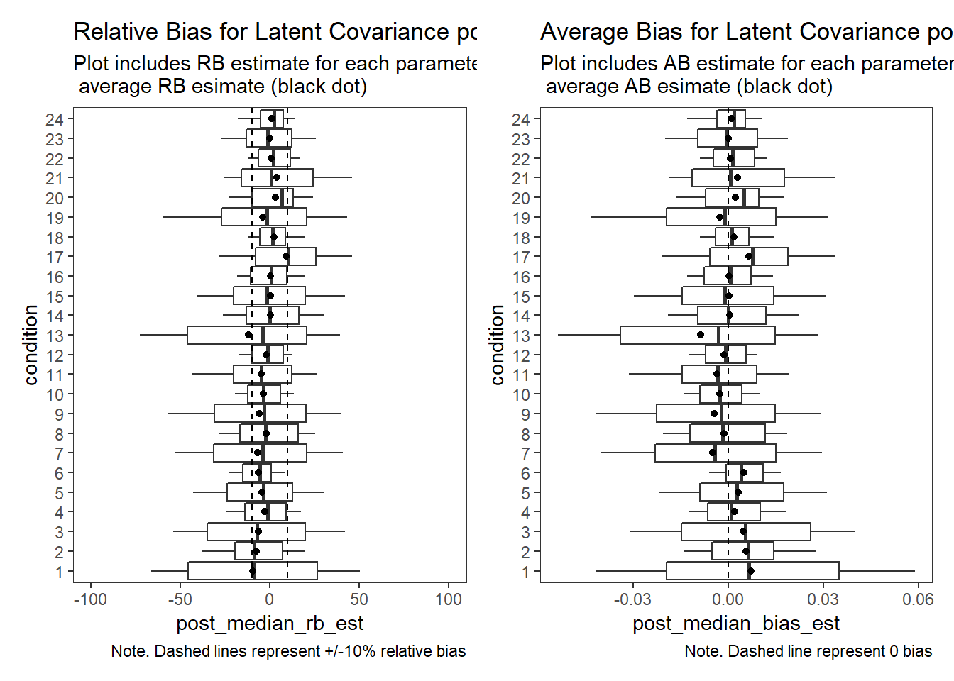
PID Relationship (\(\rho\))
param = "PID Relationship"

rb <- mydata %>%
  filter(parameter_group == "rho")

# tabular summary of relative bias
rb_tbl <- rb %>%
  group_by(condition, N_cat, N_items, N) %>%
  summarise(N_converge = n(),
            true = mean(true_value),
            avg_median_est = mean(post_q50),
            avg_mean_est = mean(post_mean),
            Post_Median_RB_Mean = mean(post_median_rb_est),
            Post_Median_RB_SD = sd(post_median_rb_est),
            Post_Mean_RB_Mean = mean(post_mean_rb_est),
            Post_Mean_RB_SD = sd(post_mean_rb_est),
            Post_Median_AB = mean(post_median_bias_est),
            Post_Mean_AB = mean(post_mean_bias_est))
`summarise()` has grouped output by 'condition', 'N_cat', 'N_items'. You can override using the `.groups` argument.kable(rb_tbl, format="html", digits=3) %>%
kable_styling(full_width = T) %>%
scroll_box(width="100%",height = "100%")| condition | N_cat | N_items | N | N_converge | true | avg_median_est | avg_mean_est | Post_Median_RB_Mean | Post_Median_RB_SD | Post_Mean_RB_Mean | Post_Mean_RB_SD | Post_Median_AB | Post_Mean_AB |
|---|---|---|---|---|---|---|---|---|---|---|---|---|---|
| 1 | 2 | 5 | 500 | 82 | 0.1 | 0.133 | 0.145 | 33.04 | 56.1 | 45.25 | 56.9 | 0.033 | 0.045 |
| 2 | 2 | 5 | 2500 | 80 | 0.1 | 0.137 | 0.139 | 37.40 | 41.2 | 38.83 | 41.2 | 0.037 | 0.039 |
| 3 | 2 | 10 | 500 | 85 | 0.1 | 0.099 | 0.102 | -1.20 | 39.6 | 2.24 | 38.6 | -0.001 | 0.002 |
| 4 | 2 | 10 | 2500 | 97 | 0.1 | 0.144 | 0.144 | 43.85 | 24.9 | 44.37 | 24.9 | 0.044 | 0.044 |
| 5 | 2 | 20 | 500 | 97 | 0.1 | 0.093 | 0.094 | -7.13 | 25.0 | -5.89 | 24.9 | -0.007 | -0.006 |
| 6 | 2 | 20 | 2500 | 100 | 0.1 | 0.136 | 0.137 | 36.33 | 16.2 | 36.65 | 16.2 | 0.036 | 0.037 |
| 7 | 5 | 5 | 500 | 91 | 0.1 | 0.136 | 0.141 | 35.60 | 61.5 | 41.07 | 59.6 | 0.036 | 0.041 |
| 8 | 5 | 5 | 2500 | 97 | 0.1 | 0.166 | 0.166 | 65.98 | 42.3 | 66.22 | 42.2 | 0.066 | 0.066 |
| 9 | 5 | 10 | 500 | 94 | 0.1 | 0.121 | 0.123 | 21.37 | 40.0 | 23.12 | 39.5 | 0.021 | 0.023 |
| 10 | 5 | 10 | 2500 | 100 | 0.1 | 0.146 | 0.147 | 46.40 | 22.2 | 46.55 | 22.1 | 0.046 | 0.047 |
| 11 | 5 | 20 | 500 | 98 | 0.1 | 0.110 | 0.111 | 10.46 | 31.6 | 11.04 | 31.4 | 0.010 | 0.011 |
| 12 | 5 | 20 | 2500 | 100 | 0.1 | 0.141 | 0.141 | 40.98 | 13.8 | 41.01 | 13.9 | 0.041 | 0.041 |
| 13 | 3 | 5 | 500 | 97 | 0.1 | 0.136 | 0.143 | 36.34 | 67.0 | 42.98 | 65.2 | 0.036 | 0.043 |
| 14 | 3 | 5 | 2500 | 98 | 0.1 | 0.164 | 0.165 | 63.92 | 39.3 | 64.79 | 39.4 | 0.064 | 0.065 |
| 15 | 3 | 10 | 500 | 99 | 0.1 | 0.126 | 0.129 | 26.41 | 44.2 | 28.59 | 43.6 | 0.026 | 0.029 |
| 16 | 3 | 10 | 2500 | 100 | 0.1 | 0.151 | 0.151 | 51.16 | 26.7 | 51.46 | 26.7 | 0.051 | 0.051 |
| 17 | 3 | 20 | 500 | 99 | 0.1 | 0.108 | 0.109 | 8.04 | 30.4 | 8.81 | 30.1 | 0.008 | 0.009 |
| 18 | 3 | 20 | 2500 | 100 | 0.1 | 0.137 | 0.137 | 36.93 | 16.7 | 37.03 | 16.8 | 0.037 | 0.037 |
| 19 | 7 | 5 | 500 | 87 | 0.1 | 0.121 | 0.126 | 20.96 | 56.2 | 25.68 | 55.1 | 0.021 | 0.026 |
| 20 | 7 | 5 | 2500 | 45 | 0.1 | 0.153 | 0.154 | 53.33 | 31.3 | 53.77 | 31.0 | 0.053 | 0.054 |
| 21 | 7 | 10 | 500 | 49 | 0.1 | 0.119 | 0.121 | 19.35 | 39.9 | 20.80 | 39.1 | 0.019 | 0.021 |
| 22 | 7 | 10 | 2500 | 49 | 0.1 | 0.141 | 0.142 | 41.47 | 18.9 | 41.63 | 18.9 | 0.041 | 0.042 |
| 23 | 7 | 20 | 500 | 50 | 0.1 | 0.110 | 0.111 | 9.96 | 28.2 | 10.53 | 28.0 | 0.010 | 0.011 |
| 24 | 7 | 20 | 2500 | 38 | 0.1 | 0.131 | 0.131 | 30.84 | 15.0 | 31.03 | 15.3 | 0.031 | 0.031 |
# visualize RB estimates
p1 <- ggplot() +
  stat_summary(
    data = rb,
    aes(x = condition, y = post_median_rb_est,
        group = condition),
    fun.data = cust.boxplot,
    geom = "boxplot"
  ) +
  geom_point(data = rb_tbl,
             aes(x = condition, y = Post_Median_RB_Mean),
             color = "black") +
  geom_abline(intercept = -10,
              slope = 0,
              linetype = "dashed") +
  geom_abline(intercept = 10,
              slope = 0,
              linetype = "dashed") +
  lims(y = c(-100, 100)) +
  coord_flip() +
  labs(
    title = paste0("Relative Bias for ", param, " posterior median"),
    subtitle = "Plot includes RB estimate for each parameter estimate (boxplot) and\n average RB esimate (black dot)",
    caption = "Note. Dashed lines represent +/-10% relative bias"
  ) +
  theme_bw() +
  theme(panel.grid = element_blank())
p2 <- ggplot() +
  stat_summary(
    data = rb,
    aes(x = condition, y = post_median_bias_est,
        group = condition),
    fun.data = cust.boxplot,
    geom = "boxplot"
  ) +
  geom_point(data = rb_tbl,
             aes(x = condition, y = Post_Median_AB),
             color = "black") +
  geom_abline(intercept = 0,
              slope = 0,
              linetype = "dashed")+
  coord_flip() +
  labs(
    title = paste0("Average Bias for ", param, " posterior median"),
    subtitle = "Plot includes AB estimate for each parameter estimate (boxplot) and\n average AB esimate (black dot)",
    caption = "Note. Dashed line represent 0 bias"
  ) +
  theme_bw() +
  theme(panel.grid = element_blank())
p1 + p2
Warning: Removed 103 rows containing non-finite values (stat_summary).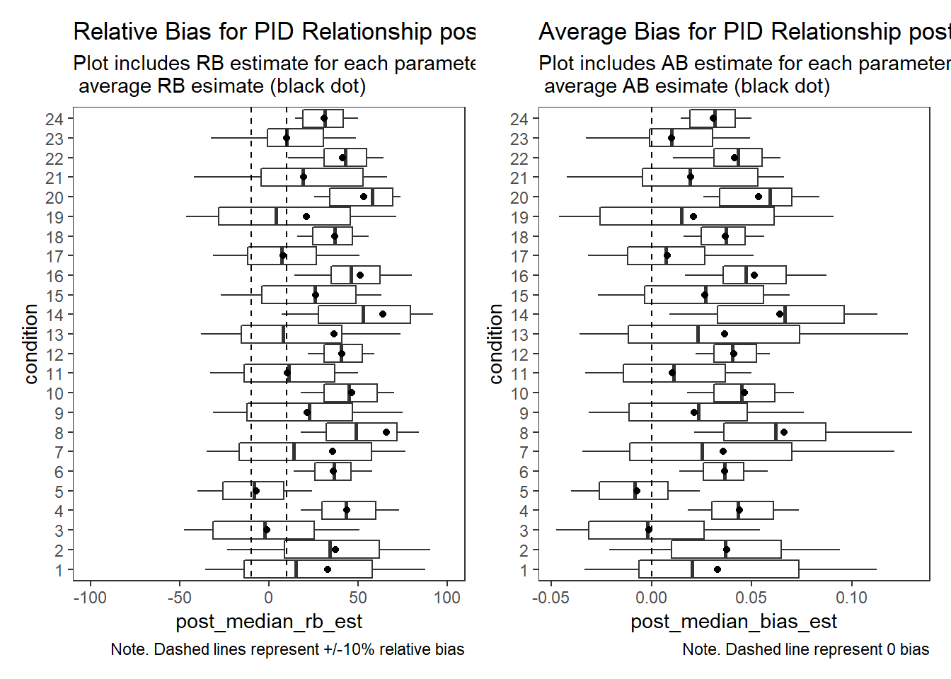
Factor Reliability (\(\omega\))
param = "RELIABILITY"

rb <- mydata %>%
  filter(parameter_group == "omega")

# tabular summary of relative bias
rb_tbl <- rb %>%
  group_by(condition, N_cat, N_items, N) %>%
  summarise(N_converge = n(),
            true = mean(true_value),
            avg_median_est = mean(post_q50),
            avg_mean_est = mean(post_mean),
            Post_Median_RB_Mean = mean(post_median_rb_est),
            Post_Median_RB_SD = sd(post_median_rb_est),
            Post_Mean_RB_Mean = mean(post_mean_rb_est),
            Post_Mean_RB_SD = sd(post_mean_rb_est),
            Post_Median_AB = mean(post_median_bias_est),
            Post_Mean_AB = mean(post_mean_bias_est))
`summarise()` has grouped output by 'condition', 'N_cat', 'N_items'. You can override using the `.groups` argument.kable(rb_tbl, format="html", digits=3) %>%
kable_styling(full_width = T) %>%
scroll_box(width="100%",height = "100%")| condition | N_cat | N_items | N | N_converge | true | avg_median_est | avg_mean_est | Post_Median_RB_Mean | Post_Median_RB_SD | Post_Mean_RB_Mean | Post_Mean_RB_SD | Post_Median_AB | Post_Mean_AB |
|---|---|---|---|---|---|---|---|---|---|---|---|---|---|
| 1 | 2 | 5 | 500 | 63 | 0.802 | 0.770 | 0.756 | -3.943 | 8.237 | -5.68 | 8.731 | -0.032 | -0.046 |
| 2 | 2 | 5 | 2500 | 78 | 0.802 | 0.767 | 0.765 | -4.310 | 3.899 | -4.65 | 3.972 | -0.035 | -0.037 |
| 3 | 2 | 10 | 500 | 88 | 0.890 | 0.876 | 0.873 | -1.532 | 2.557 | -1.88 | 2.667 | -0.014 | -0.017 |
| 4 | 2 | 10 | 2500 | 97 | 0.890 | 0.860 | 0.860 | -3.341 | 1.473 | -3.41 | 1.482 | -0.030 | -0.030 |
| 5 | 2 | 20 | 500 | 96 | 0.942 | 0.933 | 0.932 | -0.926 | 0.826 | -1.00 | 0.845 | -0.009 | -0.009 |
| 6 | 2 | 20 | 2500 | 100 | 0.942 | 0.924 | 0.924 | -1.923 | 0.412 | -1.94 | 0.413 | -0.018 | -0.018 |
| 7 | 5 | 5 | 500 | 87 | 0.802 | 0.766 | 0.763 | -4.439 | 4.466 | -4.85 | 4.594 | -0.036 | -0.039 |
| 8 | 5 | 5 | 2500 | 99 | 0.802 | 0.749 | 0.749 | -6.566 | 2.077 | -6.66 | 2.088 | -0.053 | -0.053 |
| 9 | 5 | 10 | 500 | 95 | 0.890 | 0.862 | 0.861 | -3.167 | 1.832 | -3.27 | 1.850 | -0.028 | -0.029 |
| 10 | 5 | 10 | 2500 | 97 | 0.890 | 0.856 | 0.856 | -3.848 | 0.753 | -3.86 | 0.749 | -0.034 | -0.034 |
| 11 | 5 | 20 | 500 | 98 | 0.942 | 0.926 | 0.926 | -1.691 | 0.791 | -1.72 | 0.800 | -0.016 | -0.016 |
| 12 | 5 | 20 | 2500 | 99 | 0.942 | 0.922 | 0.922 | -2.080 | 0.301 | -2.09 | 0.303 | -0.020 | -0.020 |
| 13 | 3 | 5 | 500 | 89 | 0.802 | 0.772 | 0.767 | -3.686 | 5.148 | -4.33 | 5.392 | -0.030 | -0.035 |
| 14 | 3 | 5 | 2500 | 100 | 0.802 | 0.747 | 0.746 | -6.822 | 2.694 | -6.96 | 2.706 | -0.055 | -0.056 |
| 15 | 3 | 10 | 500 | 100 | 0.890 | 0.862 | 0.861 | -3.160 | 2.175 | -3.31 | 2.216 | -0.028 | -0.029 |
| 16 | 3 | 10 | 2500 | 100 | 0.890 | 0.853 | 0.852 | -4.211 | 0.967 | -4.25 | 0.964 | -0.037 | -0.038 |
| 17 | 3 | 20 | 500 | 100 | 0.942 | 0.926 | 0.926 | -1.670 | 0.840 | -1.71 | 0.838 | -0.016 | -0.016 |
| 18 | 3 | 20 | 2500 | 99 | 0.942 | 0.920 | 0.920 | -2.352 | 0.434 | -2.36 | 0.435 | -0.022 | -0.022 |
| 19 | 7 | 5 | 500 | 81 | 0.802 | 0.776 | 0.774 | -3.182 | 4.796 | -3.51 | 4.938 | -0.026 | -0.028 |
| 20 | 7 | 5 | 2500 | 43 | 0.802 | 0.753 | 0.752 | -6.139 | 1.879 | -6.21 | 1.893 | -0.049 | -0.050 |
| 21 | 7 | 10 | 500 | 46 | 0.890 | 0.867 | 0.866 | -2.582 | 1.527 | -2.68 | 1.538 | -0.023 | -0.024 |
| 22 | 7 | 10 | 2500 | 49 | 0.890 | 0.858 | 0.858 | -3.579 | 0.765 | -3.60 | 0.761 | -0.032 | -0.032 |
| 23 | 7 | 20 | 500 | 49 | 0.942 | 0.928 | 0.928 | -1.504 | 0.623 | -1.52 | 0.625 | -0.014 | -0.014 |
| 24 | 7 | 20 | 2500 | 38 | 0.942 | 0.923 | 0.923 | -1.972 | 0.319 | -1.98 | 0.320 | -0.019 | -0.019 |
# visualize RB estimates
p1 <- ggplot() +
  stat_summary(
    data = rb,
    aes(x = condition, y = post_median_rb_est,
        group = condition),
    fun.data = cust.boxplot,
    geom = "boxplot"
  ) +
  geom_point(data = rb_tbl,
             aes(x = condition, y = Post_Median_RB_Mean),
             color = "black") +
  geom_abline(intercept = -10,
              slope = 0,
              linetype = "dashed") +
  geom_abline(intercept = 10,
              slope = 0,
              linetype = "dashed") +
  lims(y = c(-100, 100)) +
  coord_flip() +
  labs(
    title = paste0("Relative Bias for ", param, " posterior median"),
    subtitle = "Plot includes RB estimate for each parameter estimate (boxplot) and\n average RB esimate (black dot)",
    caption = "Note. Dashed lines represent +/-10% relative bias"
  ) +
  theme_bw() +
  theme(panel.grid = element_blank())
p2 <- ggplot() +
  stat_summary(
    data = rb,
    aes(x = condition, y = post_median_bias_est,
        group = condition),
    fun.data = cust.boxplot,
    geom = "boxplot"
  ) +
  geom_point(data = rb_tbl,
             aes(x = condition, y = Post_Median_AB),
             color = "black") +
  geom_abline(intercept = 0,
              slope = 0,
              linetype = "dashed")+
  coord_flip() +
  labs(
    title = paste0("Average Bias for ", param, " posterior median"),
    subtitle = "Plot includes AB estimate for each parameter estimate (boxplot) and\n average AB esimate (black dot)",
    caption = "Note. Dashed line represent 0 bias"
  ) +
  theme_bw() +
  theme(panel.grid = element_blank())
p1 + p2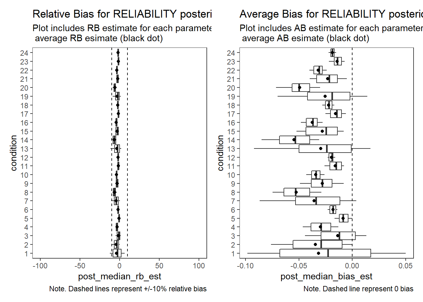
Effect of Simulated Conditions
Factor Loadings (\(\lambda\))
rb <- mydata %>%
  filter(parameter_group == "lambda") %>%
  group_by(condition, iter, N, N_cat, N_items) %>%
  summarise(
    rb_est = mean(post_median_bias_est)
  )
`summarise()` has grouped output by 'condition', 'iter', 'N', 'N_cat'. You can override using the `.groups` argument.## ANOVA on Relative Bias values
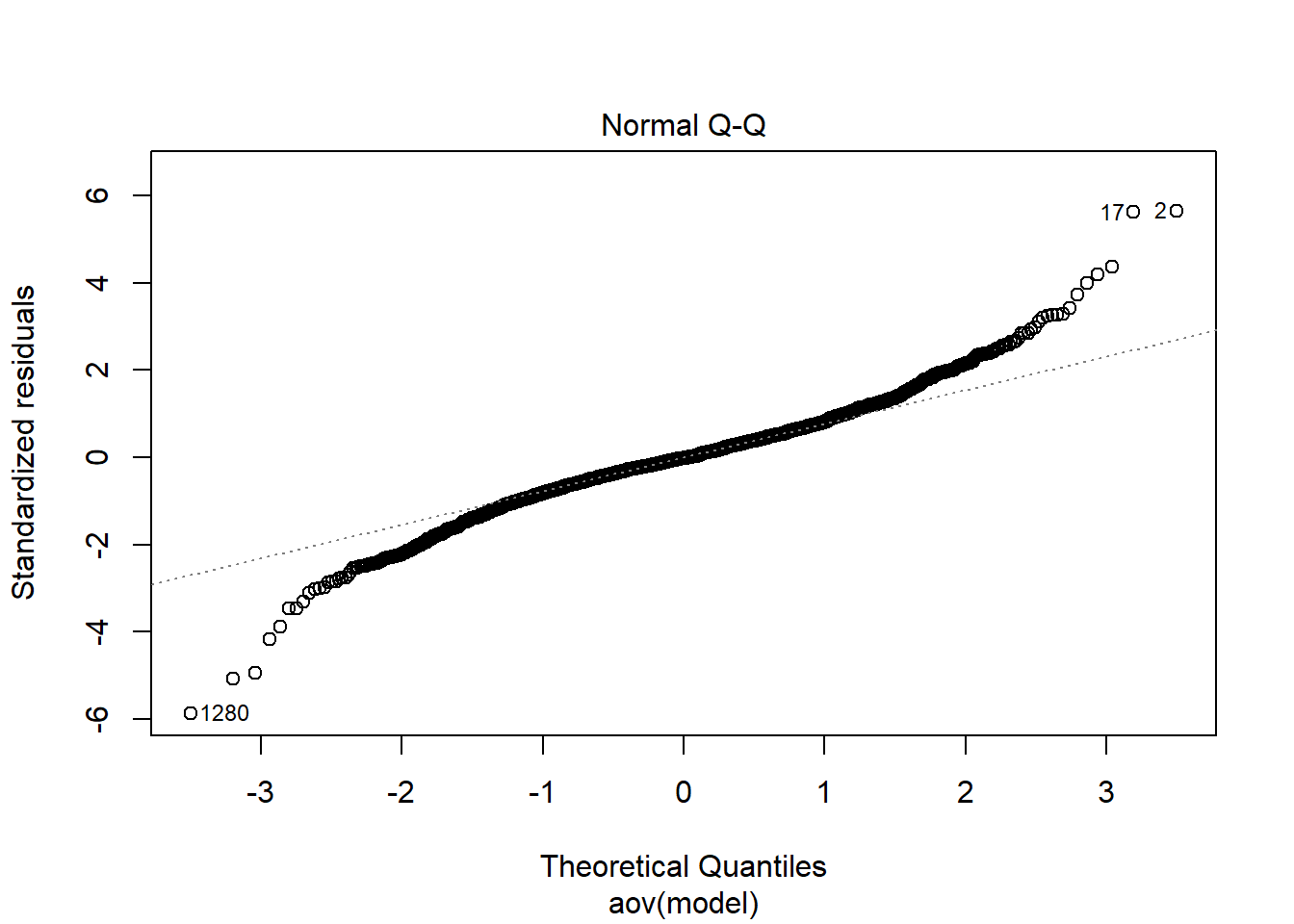
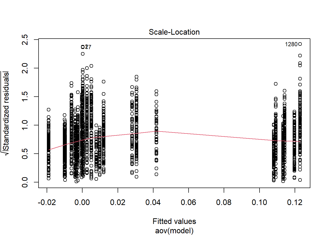
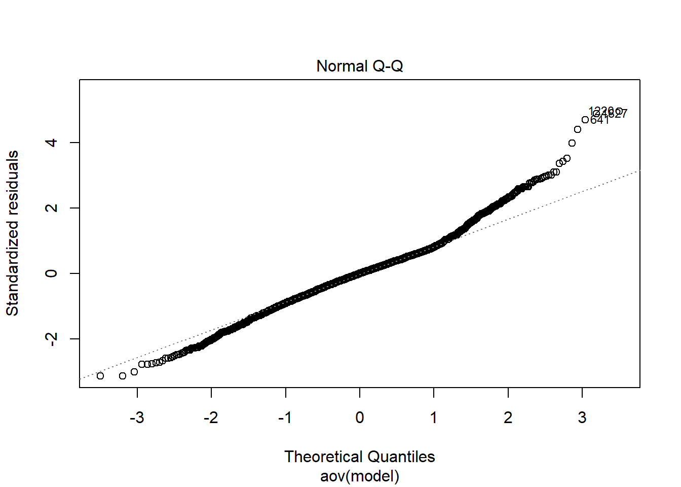
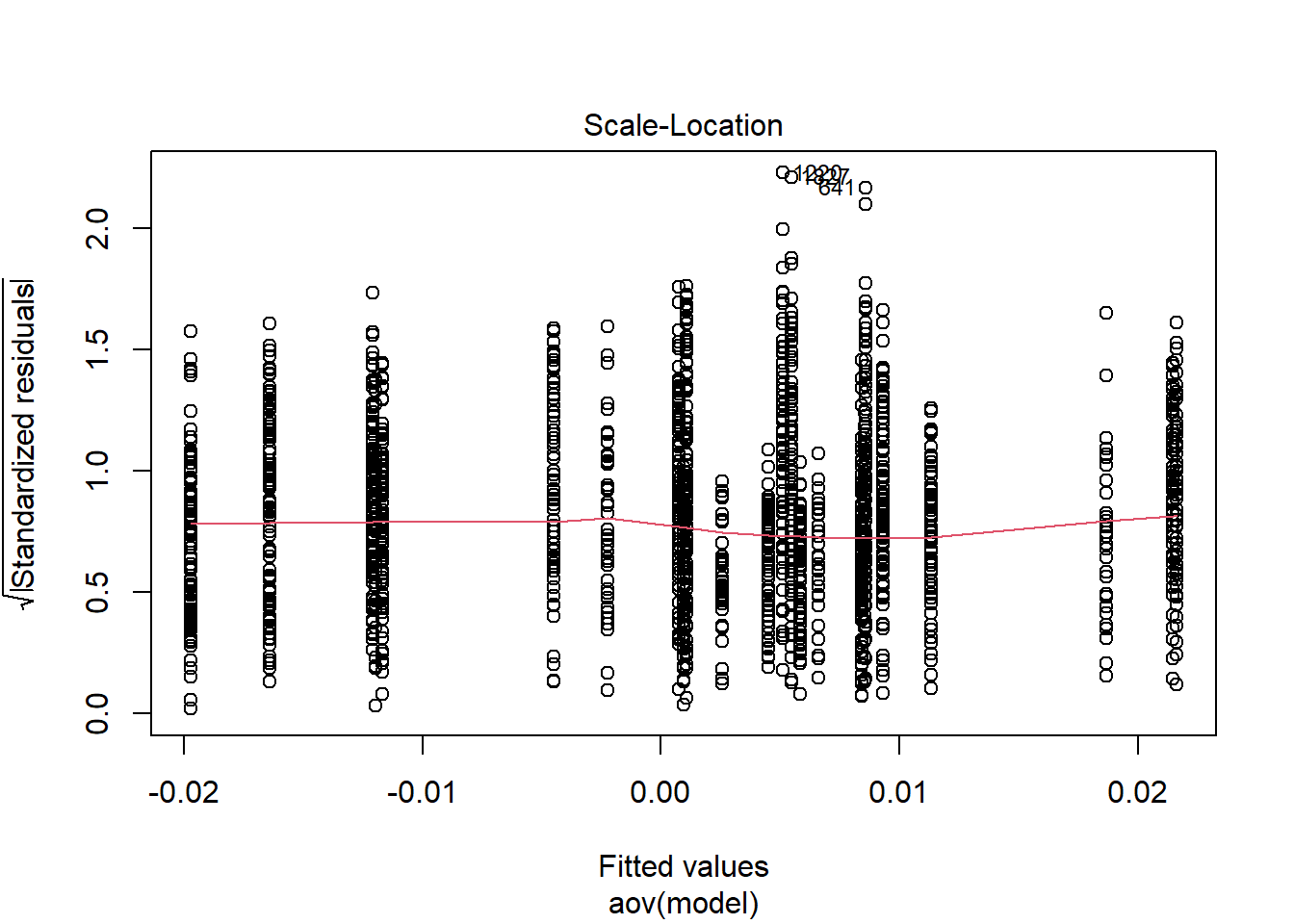
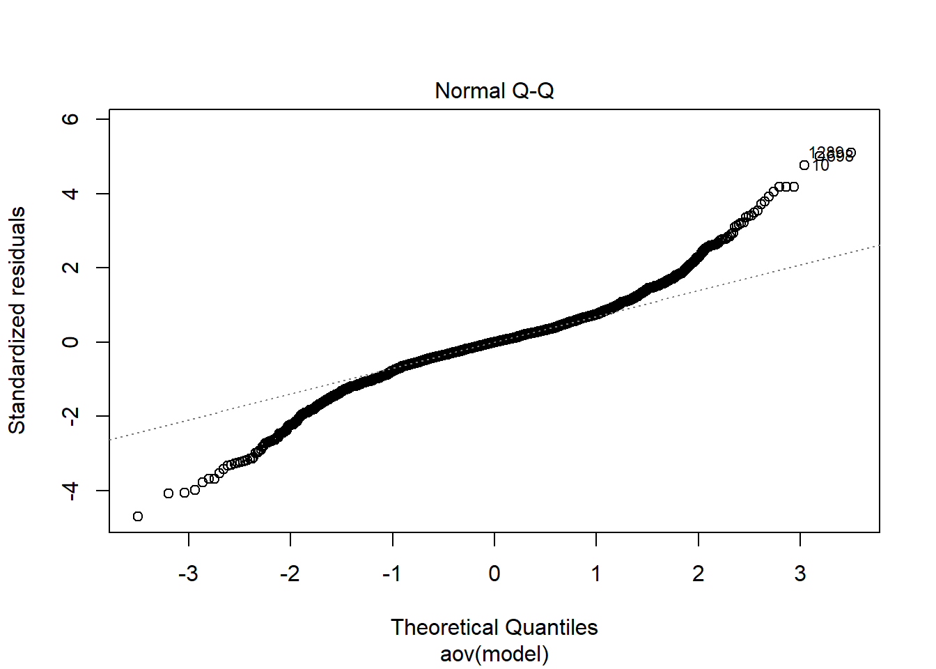
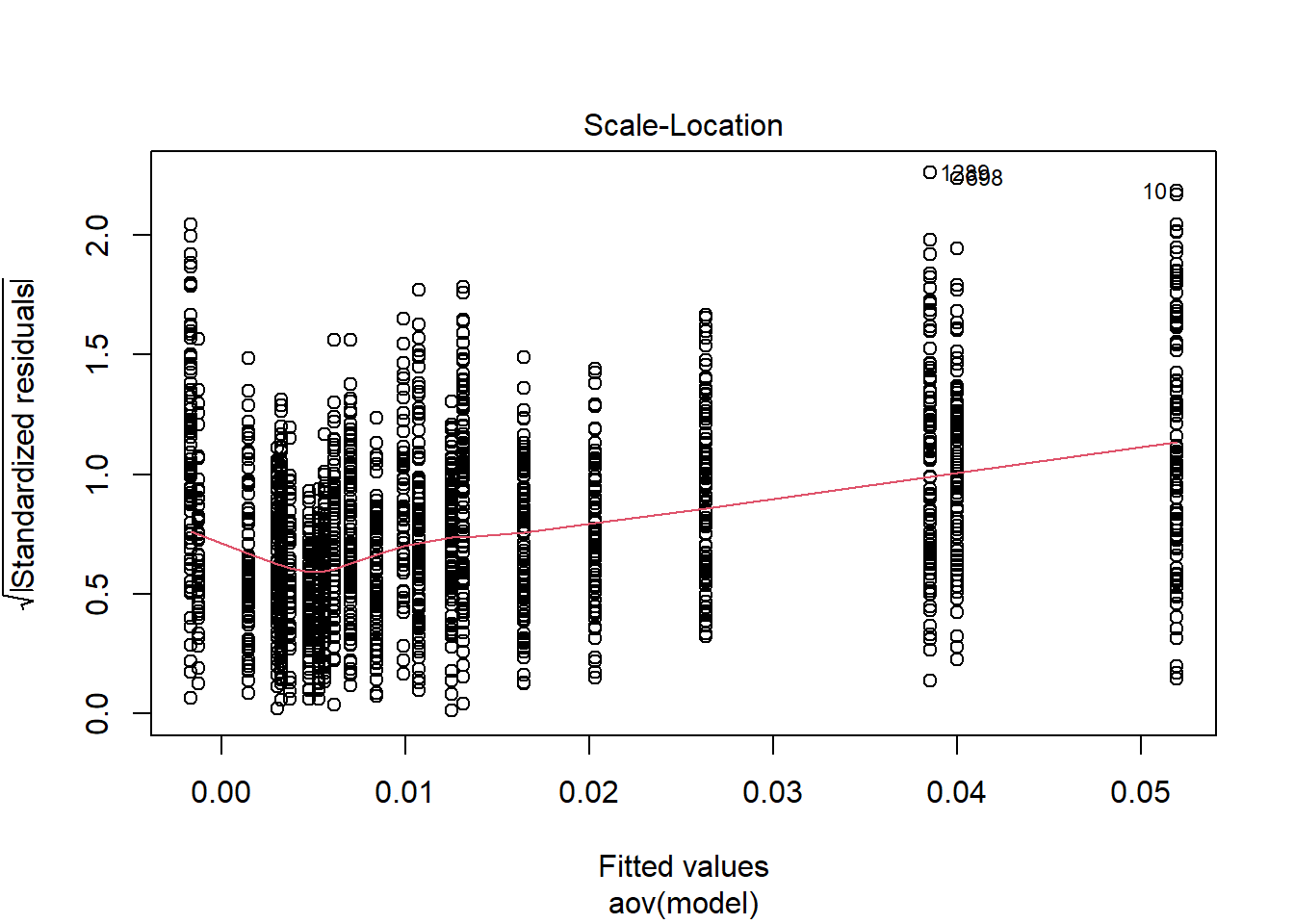
anova_assumptions_check(
dat = rb, outcome = 'rb_est',
factors = c('N_cat', 'N_items', 'N'),
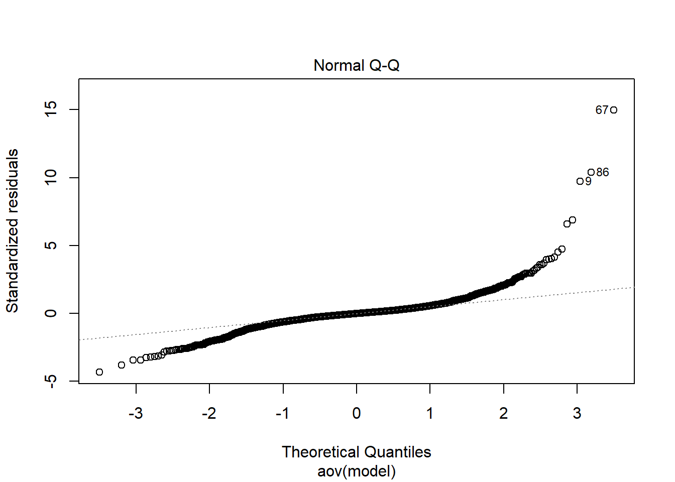
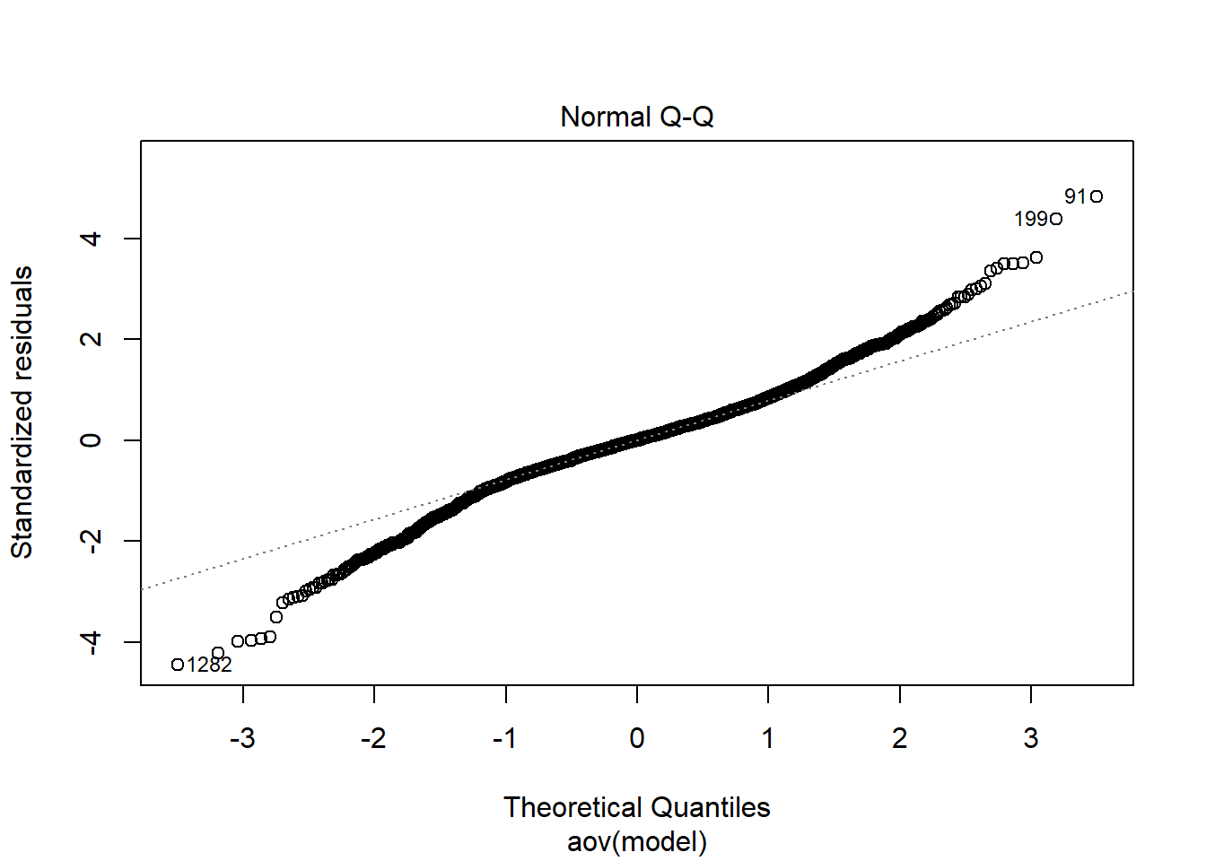
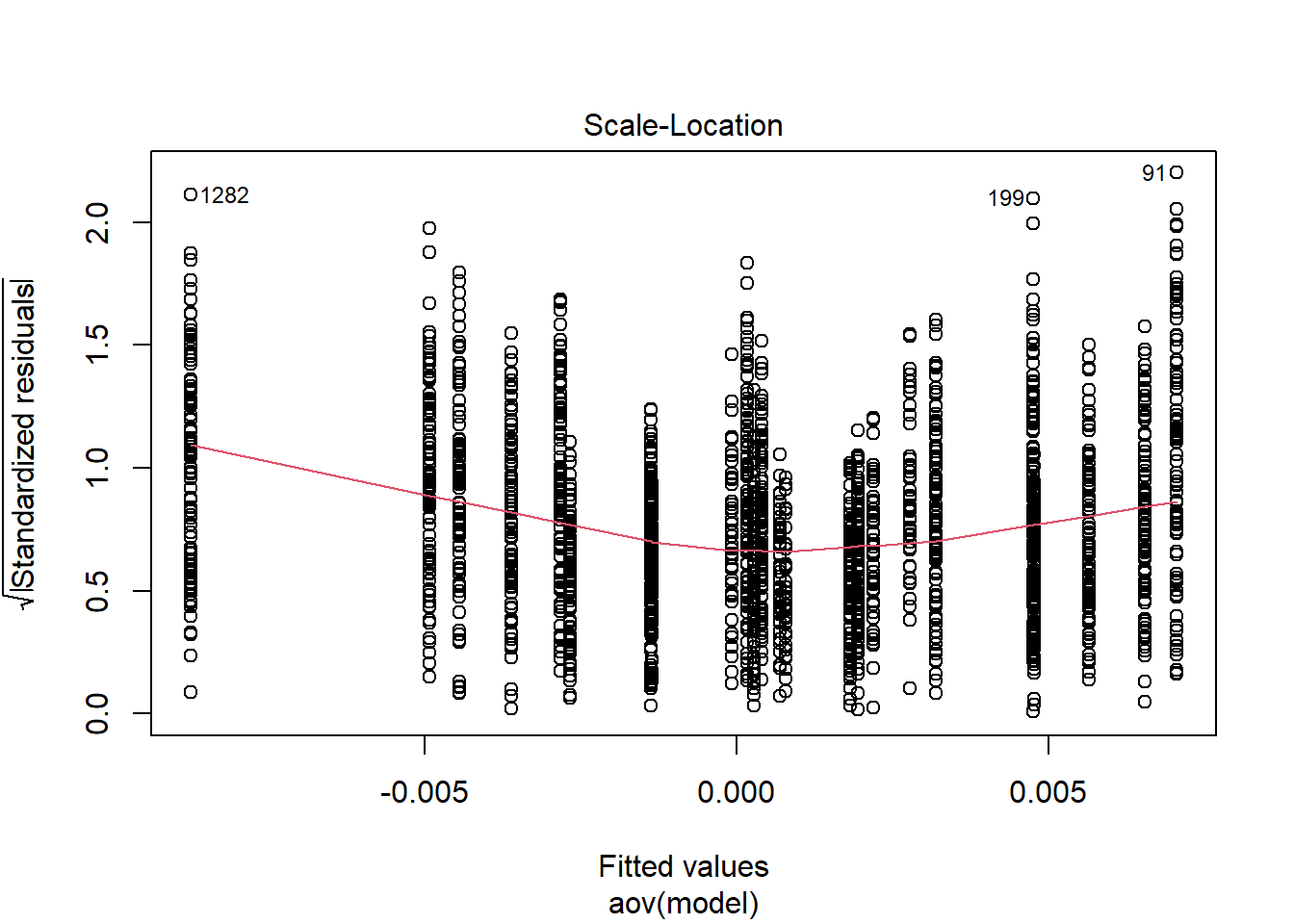
model = as.formula('rb_est ~ N_cat*N_items*N'))
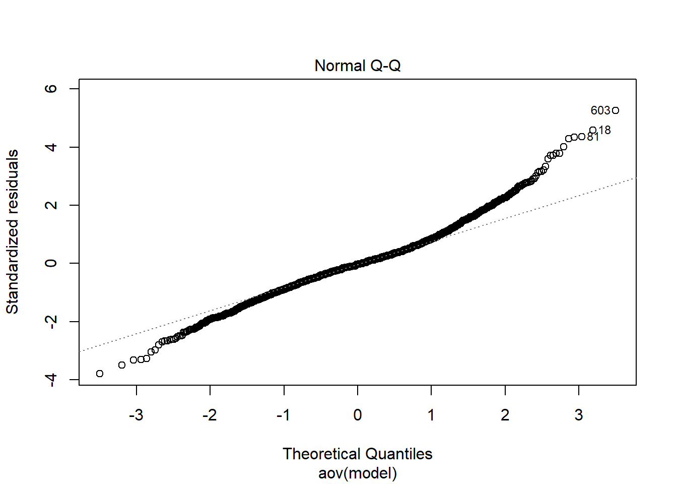
 =============================

 Tests and Plots of Normality:
 Shapiro-Wilks Test of Normality of Residuals:

    Shapiro-Wilk normality test

data:  res
W = 0.9, p-value <0.0000000000000002


 K-S Test for Normality of Residuals:
Warning in ks.test(aov.out$residuals, "pnorm", alternative = "two.sided"): ties
should not be present for the Kolmogorov-Smirnov test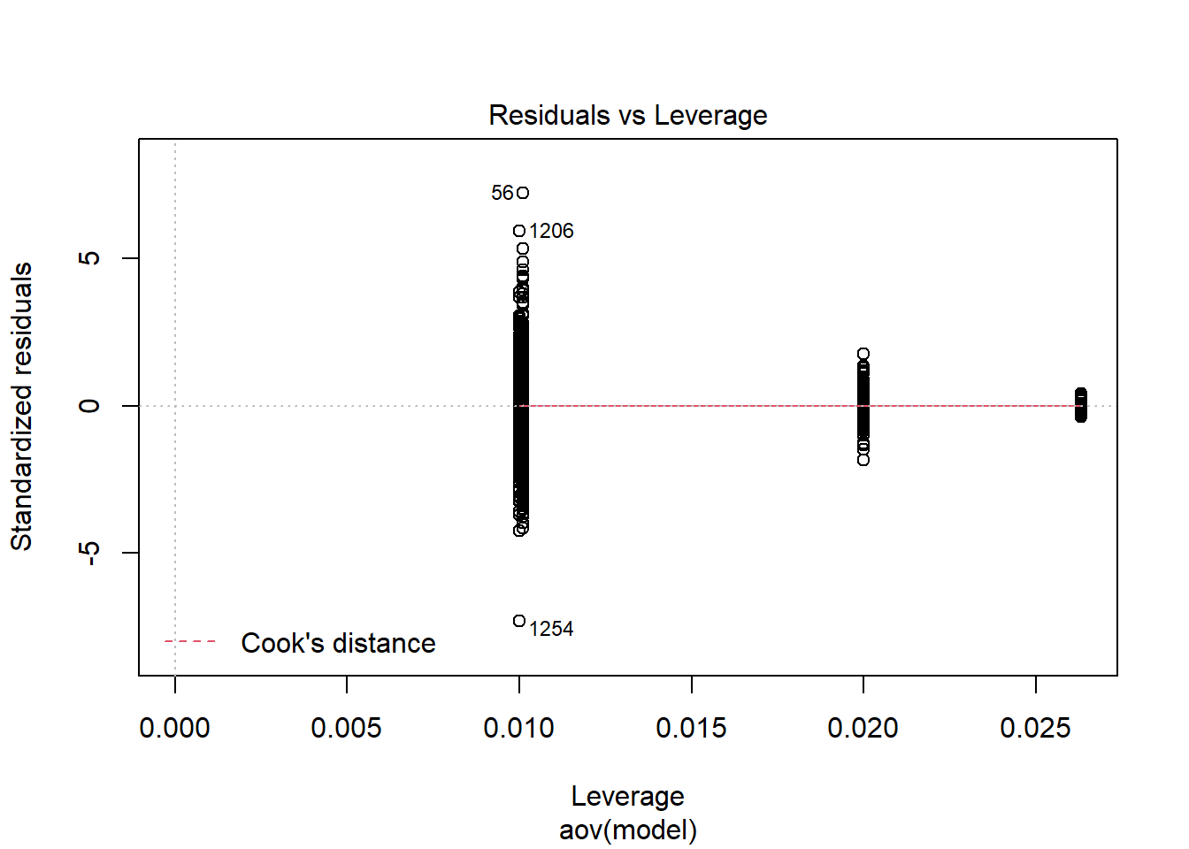
    One-sample Kolmogorov-Smirnov test

data:  aov.out$residuals
D = 0.4, p-value <0.0000000000000002
alternative hypothesis: two-sided
`stat_bin()` using `bins = 30`. Pick better value with `binwidth`.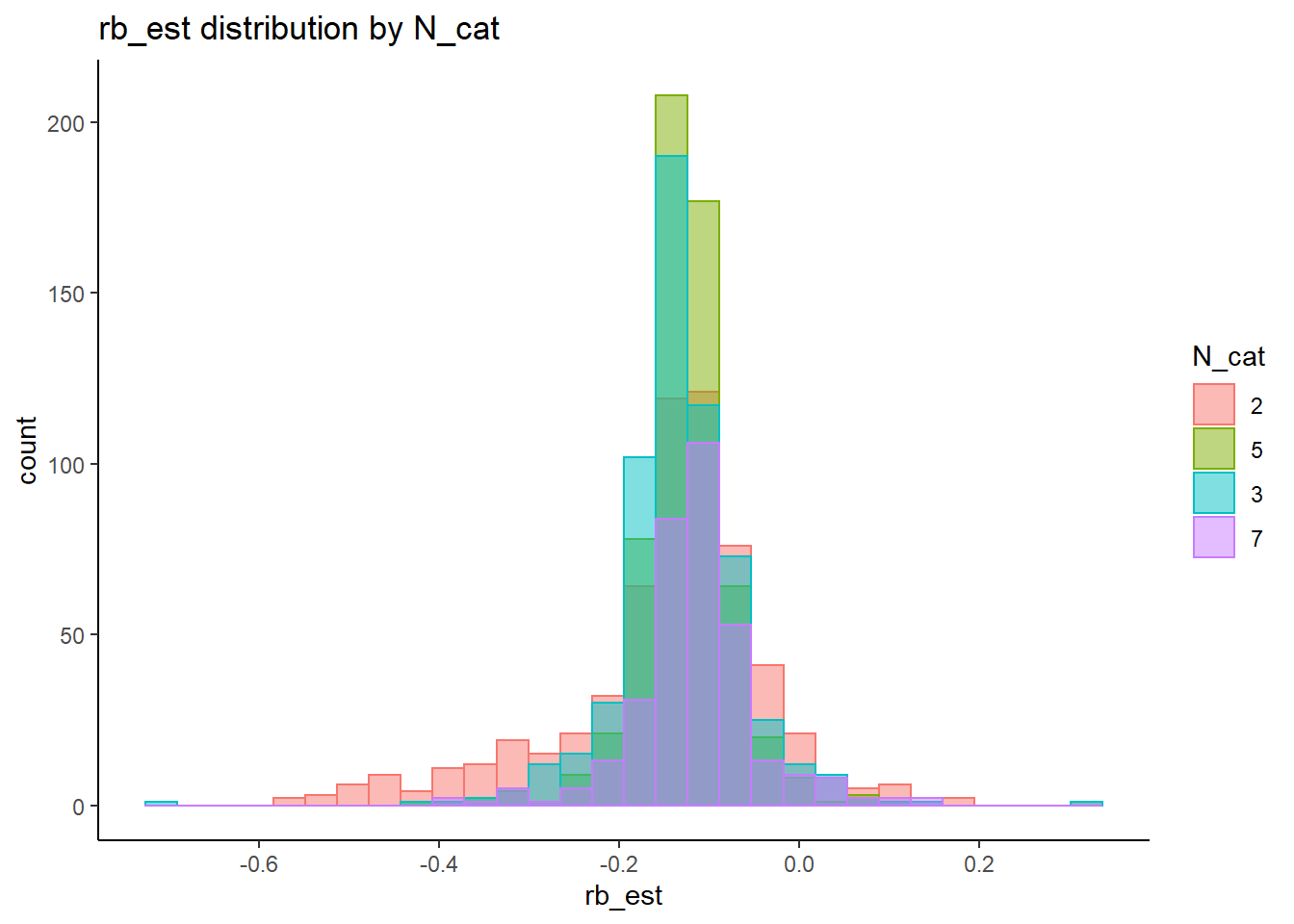
`stat_bin()` using `bins = 30`. Pick better value with `binwidth`.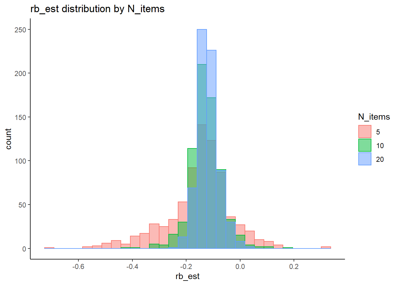
`stat_bin()` using `bins = 30`. Pick better value with `binwidth`.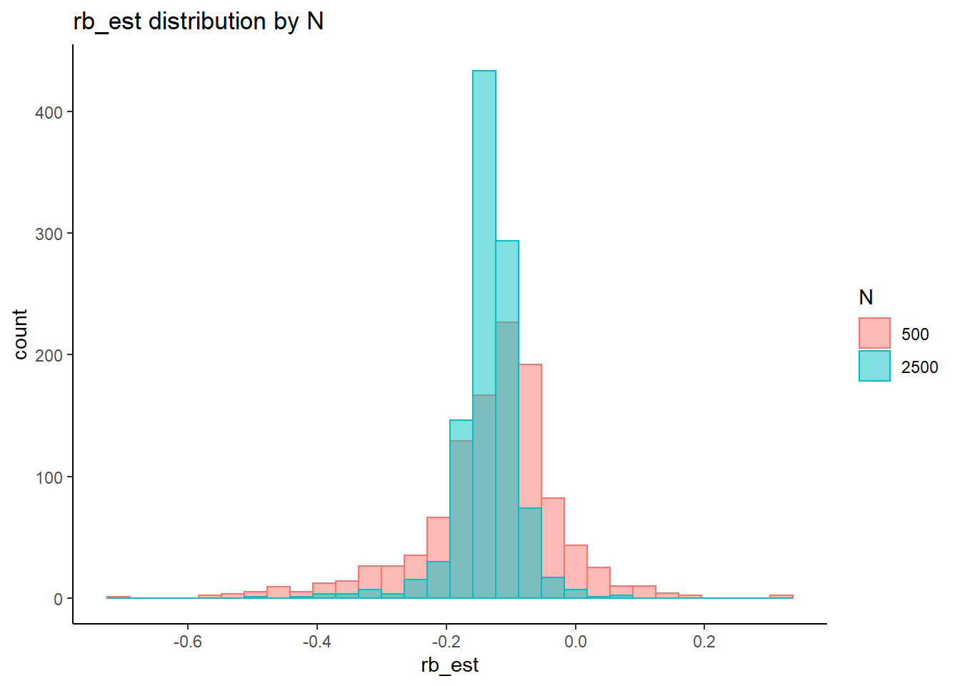
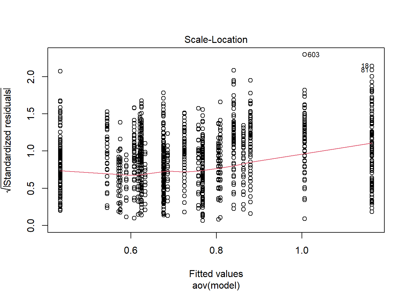
=============================
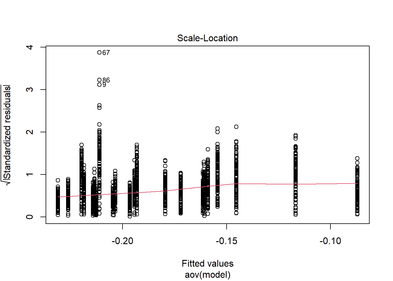
Tests of Homogeneity of Variance
Levenes Test: N_cat
Levene's Test for Homogeneity of Variance (center = "mean")
Df F value Pr(>F)
group 3 65.7 <0.0000000000000002 ***
2131
---
Signif. codes: 0 '***' 0.001 '**' 0.01 '*' 0.05 '.' 0.1 ' ' 1
Levenes Test: N_items
Levene's Test for Homogeneity of Variance (center = "mean")
Df F value Pr(>F)
group 2 203 <0.0000000000000002 ***
2132
---
Signif. codes: 0 '***' 0.001 '**' 0.01 '*' 0.05 '.' 0.1 ' ' 1
Levenes Test: N
Levene's Test for Homogeneity of Variance (center = "mean")
Df F value Pr(>F)
group 1 296 <0.0000000000000002 ***
2133
---
Signif. codes: 0 '***' 0.001 '**' 0.01 '*' 0.05 '.' 0.1 ' ' 1fit <- summary(aov(rb_est ~ N_cat*N_items*N, data=rb))
fit Df Sum Sq Mean Sq F value Pr(>F)
N_cat 3 0.22 0.0737 12.19 0.00000006560313220 ***
N_items 2 0.44 0.2216 36.65 0.00000000000000023 ***
N 1 0.01 0.0090 1.49 0.22191
N_cat:N_items 6 0.56 0.0937 15.50 < 0.0000000000000002 ***
N_cat:N 3 0.12 0.0391 6.47 0.00024 ***
N_items:N 2 0.20 0.1018 16.85 0.00000005519239311 ***
N_cat:N_items:N 6 0.18 0.0294 4.86 0.00006074631845613 ***
Residuals 2111 12.76 0.0060
---
Signif. codes: 0 '***' 0.001 '**' 0.01 '*' 0.05 '.' 0.1 ' ' 1eta_est <- (fit[[1]]$`Sum Sq`/sum(fit[[1]]$`Sum Sq`))[1:7]
cbind(omega2(fit),p_omega2(fit), eta_est) omega^2 partial-omega^2 eta_est
N_cat 0.0140 0.0155 0.015255
N_items 0.0297 0.0323 0.030573
N 0.0002 0.0002 0.000623
N_cat:N_items 0.0363 0.0392 0.038795
N_cat:N 0.0068 0.0076 0.008091
N_items:N 0.0132 0.0146 0.014052
N_cat:N_items:N 0.0097 0.0107 0.012168saved_omega[1,] <- omega2(fit)
saved_eta[1,] <- eta_estItem Thresholds (\(\tau\))
rb <- mydata %>%
filter(parameter_group == "tau") %>%
group_by(condition, iter, N, N_cat, N_items) %>%
summarise(
rb_est = mean(post_median_bias_est)
)`summarise()` has grouped output by 'condition', 'iter', 'N', 'N_cat'. You can override using the `.groups` argument.## ANOVA on Relative Bias values
anova_assumptions_check(
dat = rb, outcome = 'rb_est',
factors = c('N_cat', 'N_items', 'N'),
model = as.formula('rb_est ~ N_cat*N_items*N'))
=============================
Tests and Plots of Normality: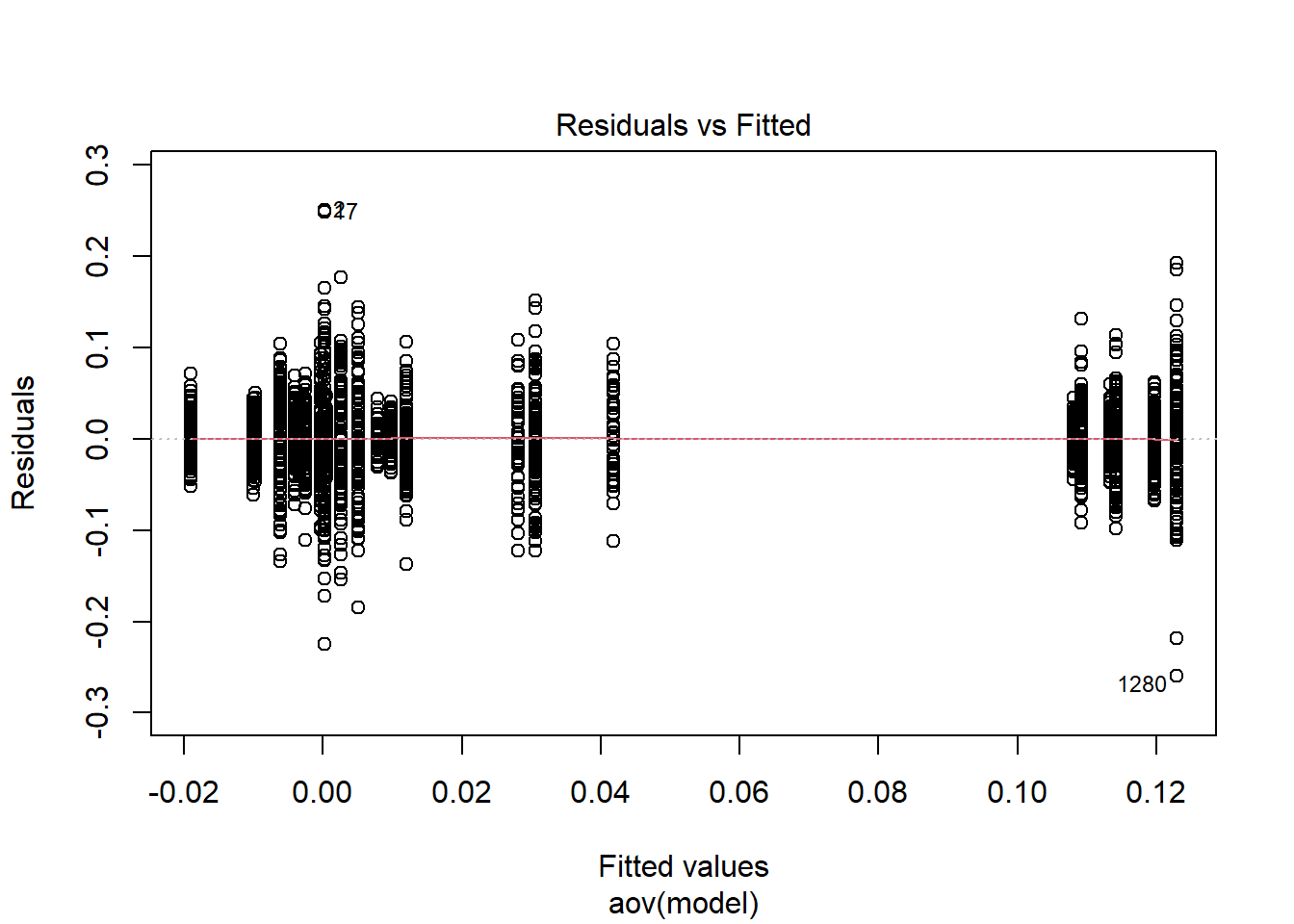
Shapiro-Wilks Test of Normality of Residuals:
Shapiro-Wilk normality test
data: res
W = 1, p-value <0.0000000000000002
K-S Test for Normality of Residuals:Warning in ks.test(aov.out$residuals, "pnorm", alternative = "two.sided"): ties
should not be present for the Kolmogorov-Smirnov test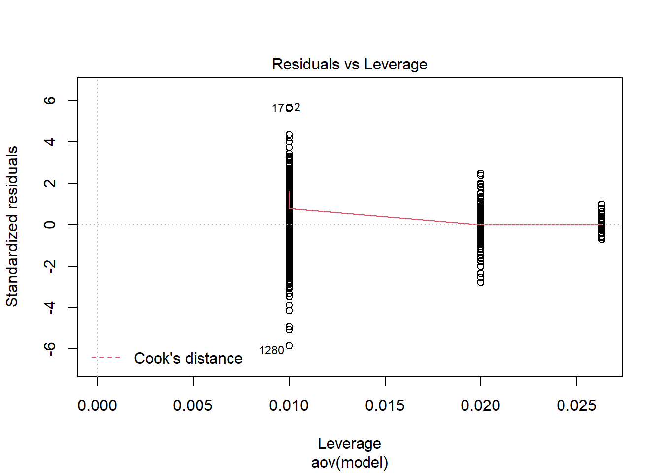
One-sample Kolmogorov-Smirnov test
data: aov.out$residuals
D = 0.4, p-value <0.0000000000000002
alternative hypothesis: two-sided`stat_bin()` using `bins = 30`. Pick better value with `binwidth`.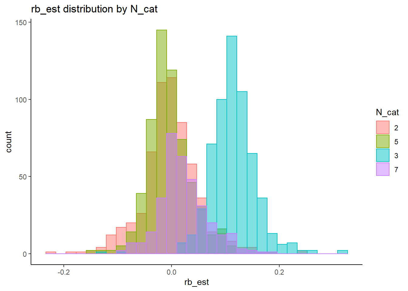
`stat_bin()` using `bins = 30`. Pick better value with `binwidth`.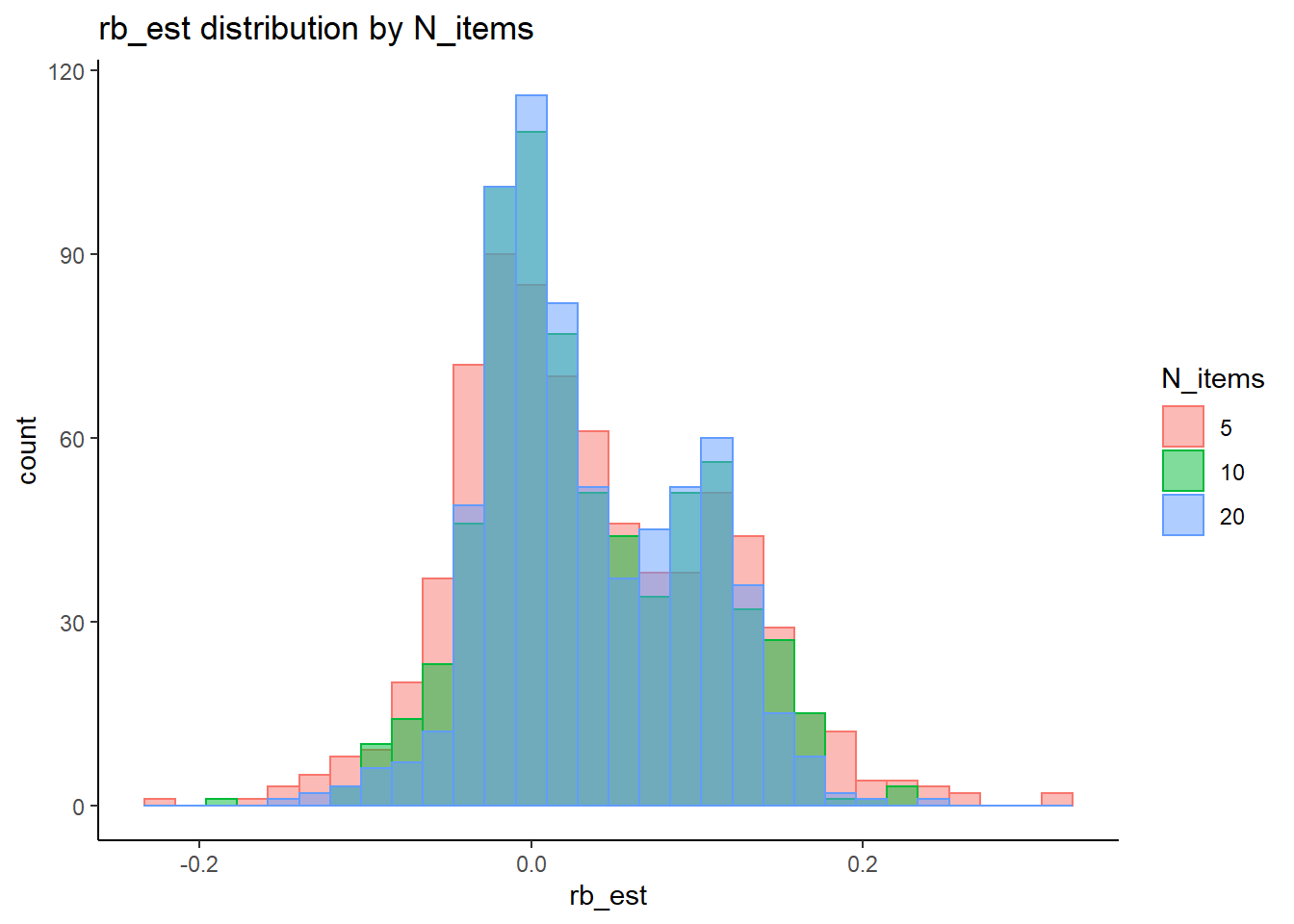
`stat_bin()` using `bins = 30`. Pick better value with `binwidth`.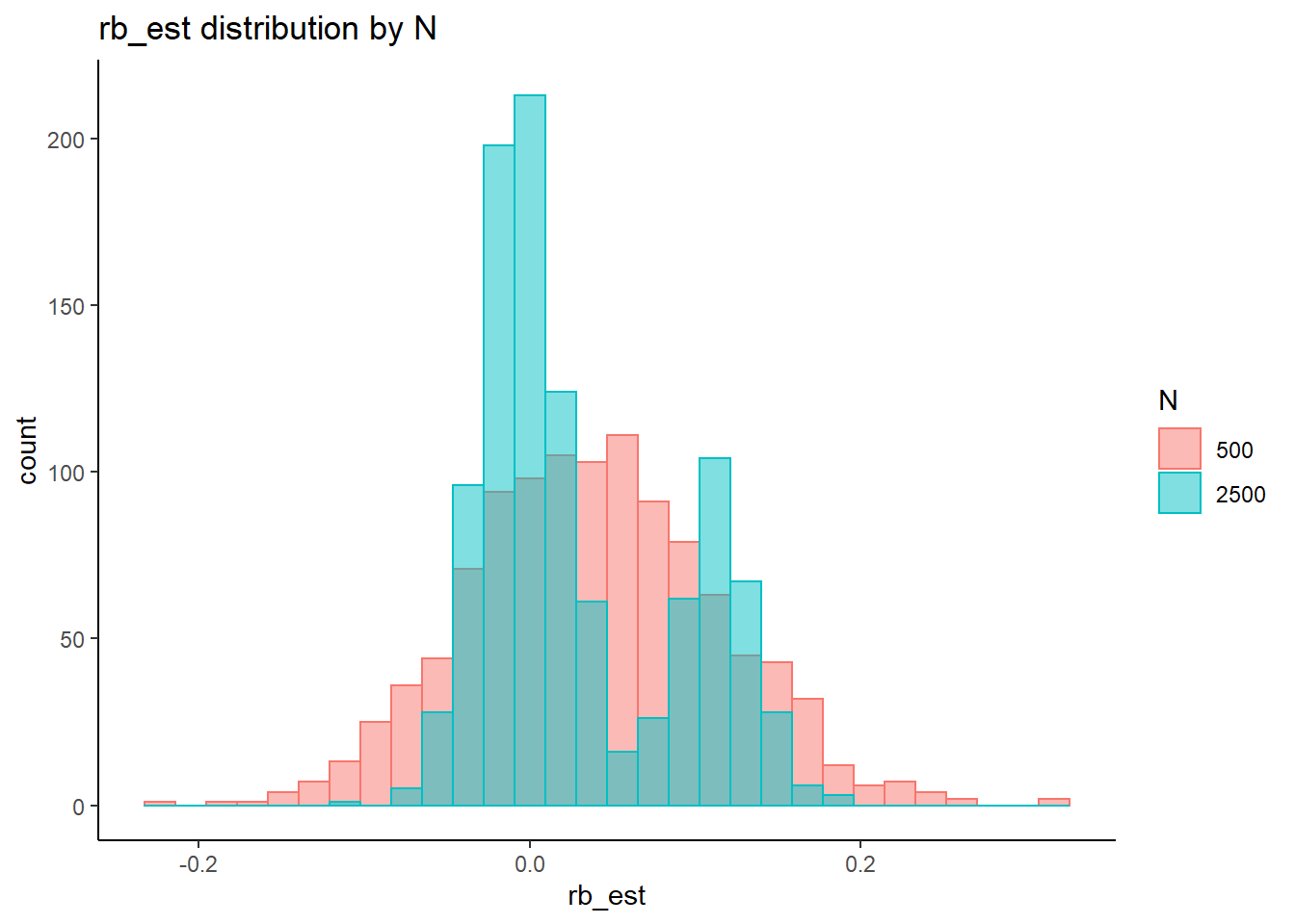
=============================
Tests of Homogeneity of Variance
Levenes Test: N_cat
Levene's Test for Homogeneity of Variance (center = "mean")
Df F value Pr(>F)
group 3 7.41 0.000062 ***
2134
---
Signif. codes: 0 '***' 0.001 '**' 0.01 '*' 0.05 '.' 0.1 ' ' 1
Levenes Test: N_items
Levene's Test for Homogeneity of Variance (center = "mean")
Df F value Pr(>F)
group 2 18.1 0.000000016 ***
2135
---
Signif. codes: 0 '***' 0.001 '**' 0.01 '*' 0.05 '.' 0.1 ' ' 1
Levenes Test: N
Levene's Test for Homogeneity of Variance (center = "mean")
Df F value Pr(>F)
group 1 32.3 0.000000015 ***
2136
---
Signif. codes: 0 '***' 0.001 '**' 0.01 '*' 0.05 '.' 0.1 ' ' 1fit <- summary(aov(rb_est ~ N_cat*N_items*N, data=rb))
fit Df Sum Sq Mean Sq F value Pr(>F)
N_cat 3 5.59 1.862 939.17 < 0.0000000000000002 ***
N_items 2 0.00 0.000 0.11 0.896
N 1 0.06 0.058 29.38 0.000000066 ***
N_cat:N_items 6 0.03 0.005 2.65 0.015 *
N_cat:N 3 0.05 0.017 8.52 0.000012707 ***
N_items:N 2 0.00 0.001 0.37 0.692
N_cat:N_items:N 6 0.01 0.002 0.89 0.501
Residuals 2114 4.19 0.002
---
Signif. codes: 0 '***' 0.001 '**' 0.01 '*' 0.05 '.' 0.1 ' ' 1eta_est <- (fit[[1]]$`Sum Sq`/sum(fit[[1]]$`Sum Sq`))[1:7]
cbind(omega2(fit),p_omega2(fit), eta_est) omega^2 partial-omega^2 eta_est
N_cat 0.5618 0.5683 0.5625320
N_items -0.0004 -0.0008 0.0000437
N 0.0057 0.0131 0.0058656
N_cat:N_items 0.0020 0.0046 0.0031735
N_cat:N 0.0045 0.0104 0.0051015
N_items:N -0.0003 -0.0006 0.0001468
N_cat:N_items:N -0.0001 -0.0003 0.0010667saved_omega[2,] <- omega2(fit)
saved_eta[2,] <- eta_estLatent Response Variance (\(\theta\))
rb <- mydata %>%
filter(parameter_group == "theta") %>%
group_by(condition, iter, N, N_cat, N_items) %>%
summarise(
rb_est = mean(post_median_bias_est)
)`summarise()` has grouped output by 'condition', 'iter', 'N', 'N_cat'. You can override using the `.groups` argument.## ANOVA on Relative Bias values
anova_assumptions_check(
dat = rb, outcome = 'rb_est',
factors = c('N_cat', 'N_items', 'N'),
model = as.formula('rb_est ~ N_cat*N_items*N'))
=============================
Tests and Plots of Normality: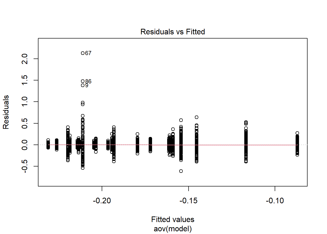
Shapiro-Wilks Test of Normality of Residuals:
Shapiro-Wilk normality test
data: res
W = 0.8, p-value <0.0000000000000002
K-S Test for Normality of Residuals:Warning in ks.test(aov.out$residuals, "pnorm", alternative = "two.sided"): ties
should not be present for the Kolmogorov-Smirnov test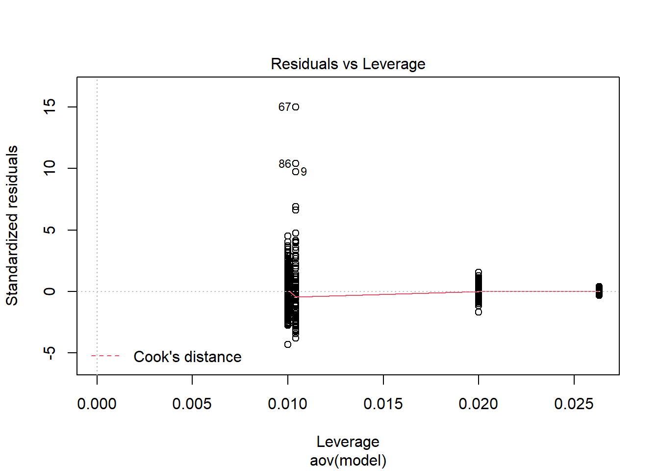
One-sample Kolmogorov-Smirnov test
data: aov.out$residuals
D = 0.4, p-value <0.0000000000000002
alternative hypothesis: two-sided`stat_bin()` using `bins = 30`. Pick better value with `binwidth`.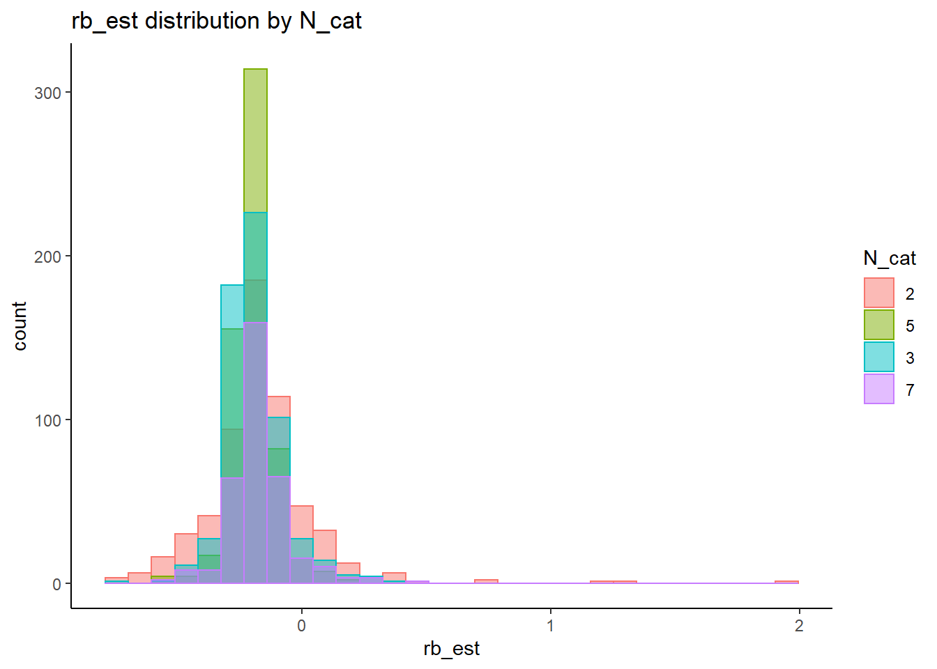
`stat_bin()` using `bins = 30`. Pick better value with `binwidth`.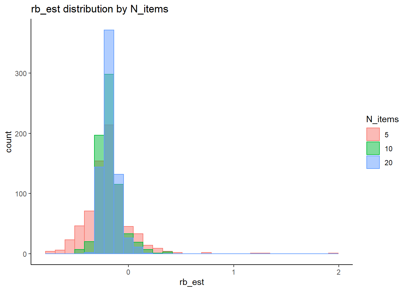
`stat_bin()` using `bins = 30`. Pick better value with `binwidth`.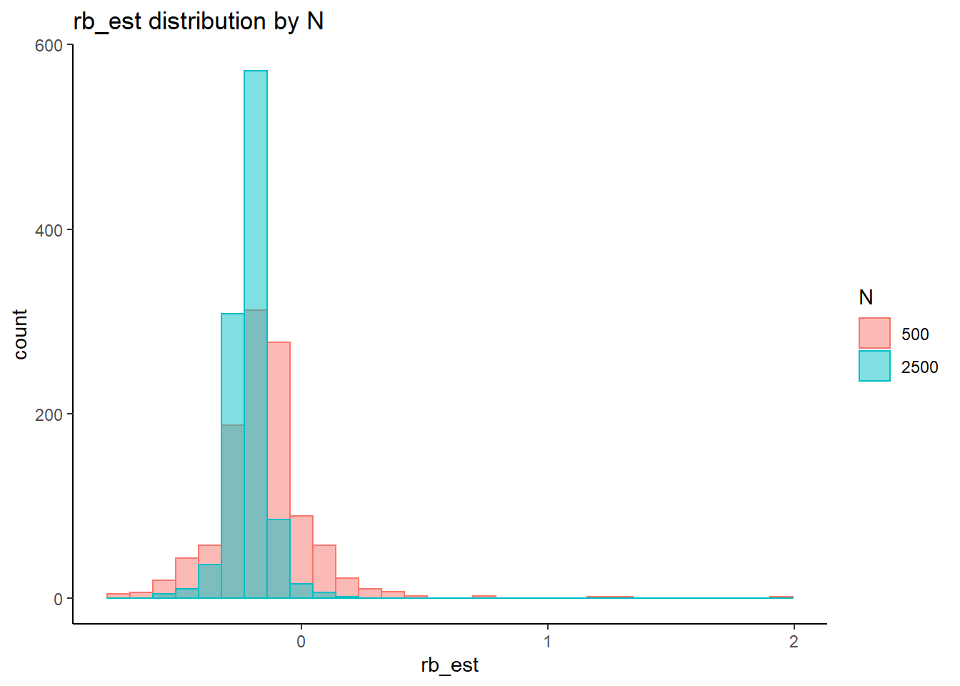
=============================
Tests of Homogeneity of Variance
Levenes Test: N_cat
Levene's Test for Homogeneity of Variance (center = "mean")
Df F value Pr(>F)
group 3 55 <0.0000000000000002 ***
2129
---
Signif. codes: 0 '***' 0.001 '**' 0.01 '*' 0.05 '.' 0.1 ' ' 1
Levenes Test: N_items
Levene's Test for Homogeneity of Variance (center = "mean")
Df F value Pr(>F)
group 2 112 <0.0000000000000002 ***
2130
---
Signif. codes: 0 '***' 0.001 '**' 0.01 '*' 0.05 '.' 0.1 ' ' 1
Levenes Test: N
Levene's Test for Homogeneity of Variance (center = "mean")
Df F value Pr(>F)
group 1 250 <0.0000000000000002 ***
2131
---
Signif. codes: 0 '***' 0.001 '**' 0.01 '*' 0.05 '.' 0.1 ' ' 1fit <- summary(aov(rb_est ~ N_cat*N_items*N, data=rb))
eta_est <- (fit[[1]]$`Sum Sq`/sum(fit[[1]]$`Sum Sq`))[1:7]
cbind(omega2(fit),p_omega2(fit), eta_est)
omega^2 partial-omega^2 eta_est
N_cat 0.0049 0.0051 0.00620
N_items 0.0018 0.0019 0.00272
N 0.0342 0.0348 0.03462
N_cat:N_items 0.0079 0.0082 0.01055
N_cat:N 0.0013 0.0014 0.00264
N_items:N 0.0013 0.0014 0.00218
N_cat:N_items:N 0.0012 0.0013 0.00387saved_omega[3,] <- omega2(fit)
saved_eta[3,] <- eta_estResponse Time Intercepts (\(\beta_{lrt}\))
rb <- mydata %>%
filter(parameter_group == "beta_lrt") %>%
group_by(condition, iter, N, N_cat, N_items) %>%
summarise(
rb_est = mean(post_median_bias_est)
)`summarise()` has grouped output by 'condition', 'iter', 'N', 'N_cat'. You can override using the `.groups` argument.## ANOVA on Relative Bias values
anova_assumptions_check(
dat = rb, outcome = 'rb_est',
factors = c('N_cat', 'N_items', 'N'),
model = as.formula('rb_est ~ N_cat*N_items*N'))
 =============================

 Tests and Plots of Normality: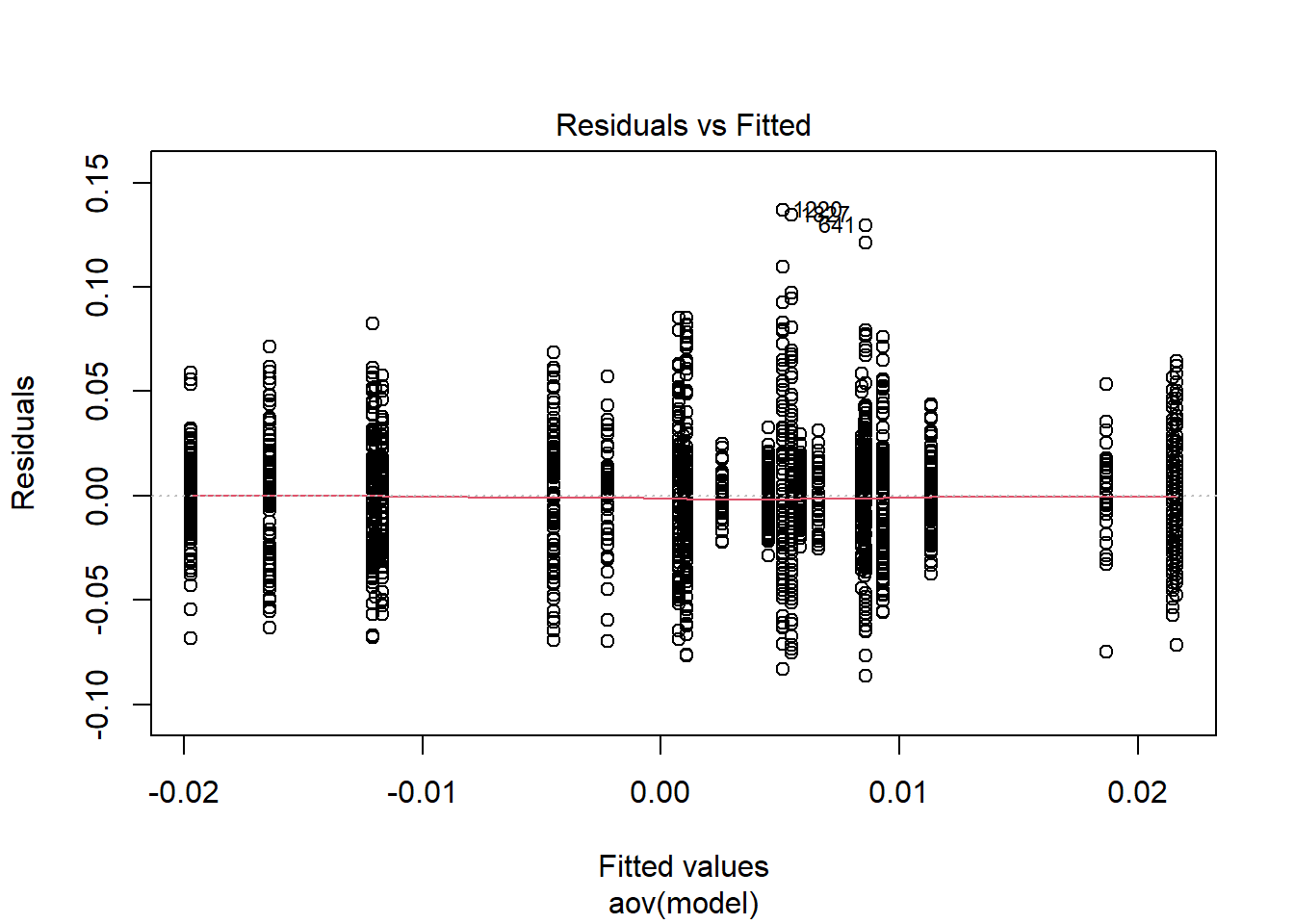
Shapiro-Wilks Test of Normality of Residuals:
Shapiro-Wilk normality test
data: res
W = 1, p-value = 0.0000000000000003
K-S Test for Normality of Residuals:Warning in ks.test(aov.out$residuals, "pnorm", alternative = "two.sided"): ties
should not be present for the Kolmogorov-Smirnov test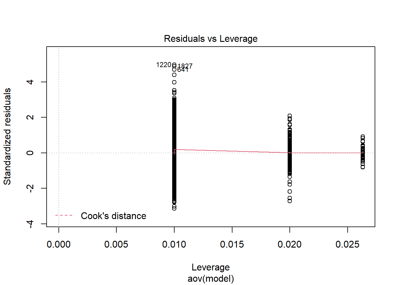
One-sample Kolmogorov-Smirnov test
data: aov.out$residuals
D = 0.5, p-value <0.0000000000000002
alternative hypothesis: two-sided`stat_bin()` using `bins = 30`. Pick better value with `binwidth`.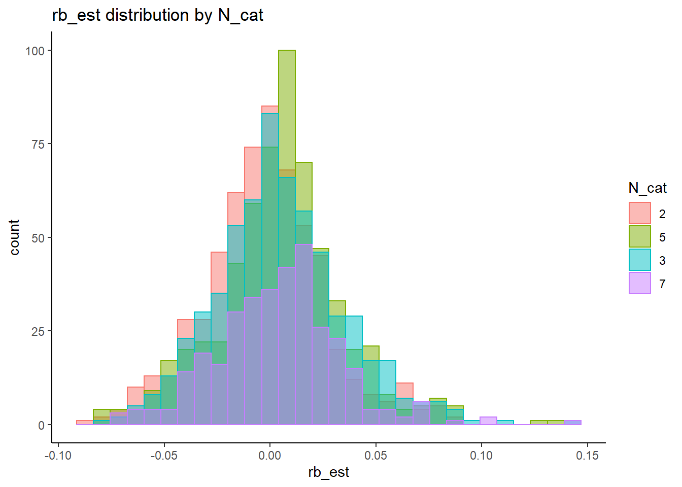
`stat_bin()` using `bins = 30`. Pick better value with `binwidth`.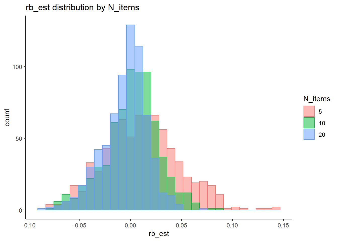
`stat_bin()` using `bins = 30`. Pick better value with `binwidth`.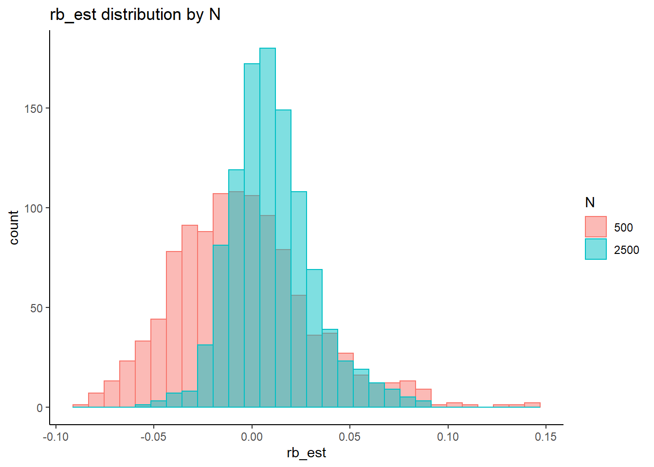
=============================
Tests of Homogeneity of Variance
Levenes Test: N_cat
Levene's Test for Homogeneity of Variance (center = "mean")
Df F value Pr(>F)
group 3 0.67 0.57
2134
Levenes Test: N_items
Levene's Test for Homogeneity of Variance (center = "mean")
Df F value Pr(>F)
group 2 83.7 <0.0000000000000002 ***
2135
---
Signif. codes: 0 '***' 0.001 '**' 0.01 '*' 0.05 '.' 0.1 ' ' 1
Levenes Test: N
Levene's Test for Homogeneity of Variance (center = "mean")
Df F value Pr(>F)
group 1 188 <0.0000000000000002 ***
2136
---
Signif. codes: 0 '***' 0.001 '**' 0.01 '*' 0.05 '.' 0.1 ' ' 1fit <- summary(aov(rb_est ~ N_cat*N_items*N, data=rb))
fit Df Sum Sq Mean Sq F value Pr(>F)
N_cat 3 0.019 0.0063 8.16 0.000021 ***
N_items 2 0.097 0.0483 62.85 < 0.0000000000000002 ***
N 1 0.121 0.1213 157.92 < 0.0000000000000002 ***
N_cat:N_items 6 0.005 0.0008 1.05 0.392
N_cat:N 3 0.004 0.0012 1.57 0.194
N_items:N 2 0.002 0.0011 1.42 0.242
N_cat:N_items:N 6 0.009 0.0015 1.90 0.077 .
Residuals 2114 1.624 0.0008
---
Signif. codes: 0 '***' 0.001 '**' 0.01 '*' 0.05 '.' 0.1 ' ' 1eta_est <- (fit[[1]]$`Sum Sq`/sum(fit[[1]]$`Sum Sq`))[1:7]
cbind(omega2(fit),p_omega2(fit), eta_est) omega^2 partial-omega^2 eta_est
N_cat 0.0088 0.0099 0.01000
N_items 0.0505 0.0547 0.05136
N 0.0641 0.0684 0.06453
N_cat:N_items 0.0001 0.0001 0.00257
N_cat:N 0.0007 0.0008 0.00193
N_items:N 0.0003 0.0004 0.00116
N_cat:N_items:N 0.0022 0.0025 0.00466saved_omega[4,] <- omega2(fit)
saved_eta[4,] <- eta_estResponse Time Precision (\(\sigma_{lrt}\))
rb <- mydata %>%
filter(parameter_group == "sigma_lrt") %>%
group_by(condition, iter, N, N_cat, N_items) %>%
summarise(
rb_est = mean(post_median_bias_est)
)`summarise()` has grouped output by 'condition', 'iter', 'N', 'N_cat'. You can override using the `.groups` argument.## ANOVA on Relative Bias values
anova_assumptions_check(
dat = rb, outcome = 'rb_est',
factors = c('N_cat', 'N_items', 'N'),
model = as.formula('rb_est ~ N_cat*N_items*N'))
=============================
Tests and Plots of Normality: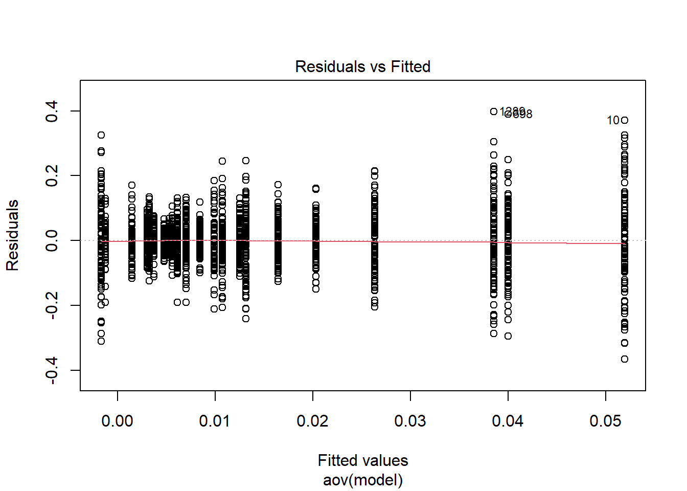
 Shapiro-Wilks Test of Normality of Residuals:

    Shapiro-Wilk normality test

data:  res
W = 1, p-value <0.0000000000000002


 K-S Test for Normality of Residuals:
Warning in ks.test(aov.out$residuals, "pnorm", alternative = "two.sided"): ties
should not be present for the Kolmogorov-Smirnov test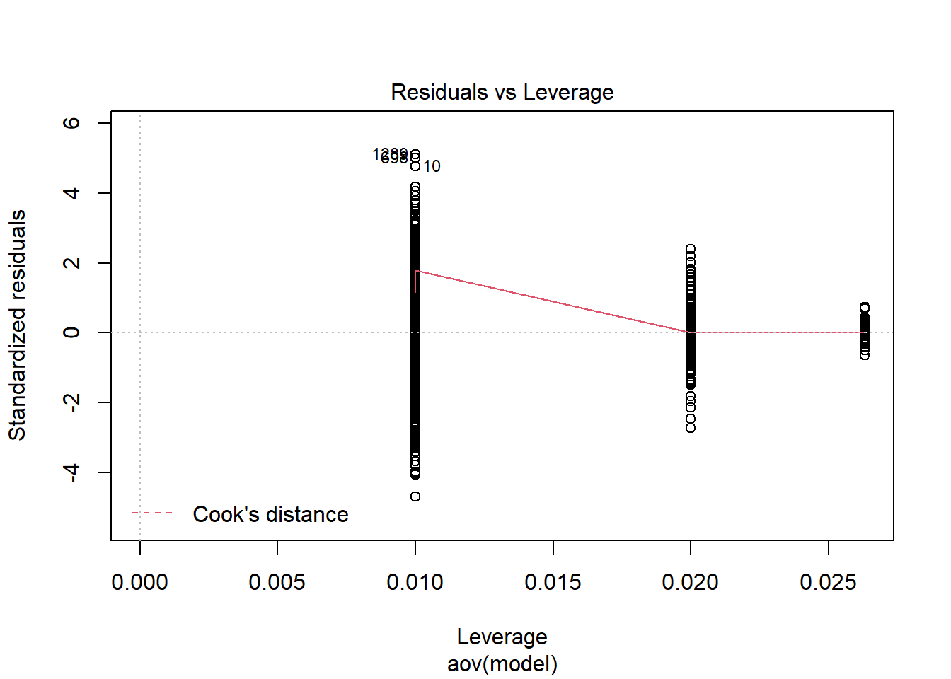
    One-sample Kolmogorov-Smirnov test

data:  aov.out$residuals
D = 0.4, p-value <0.0000000000000002
alternative hypothesis: two-sided
`stat_bin()` using `bins = 30`. Pick better value with `binwidth`.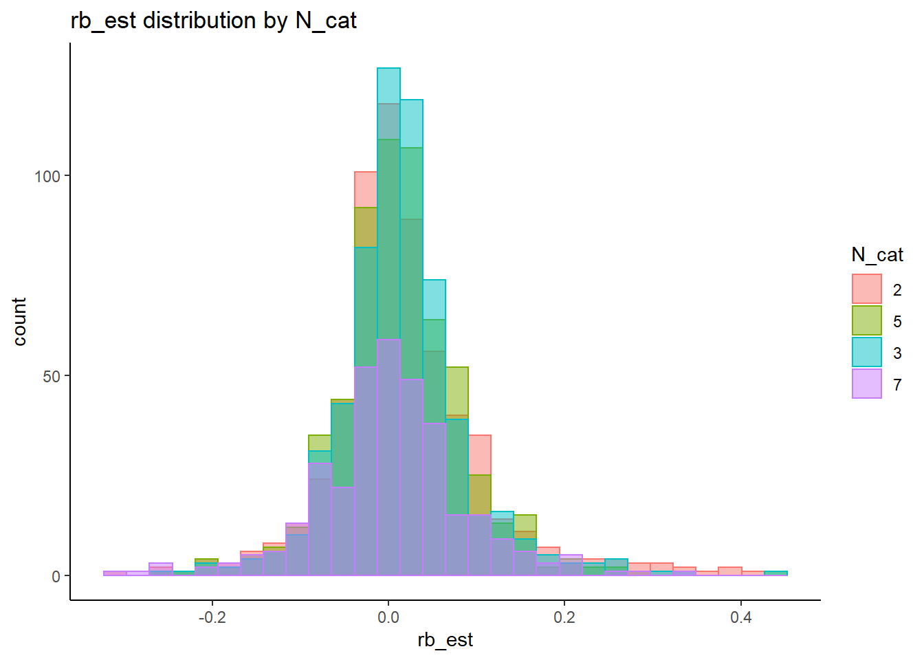
`stat_bin()` using `bins = 30`. Pick better value with `binwidth`.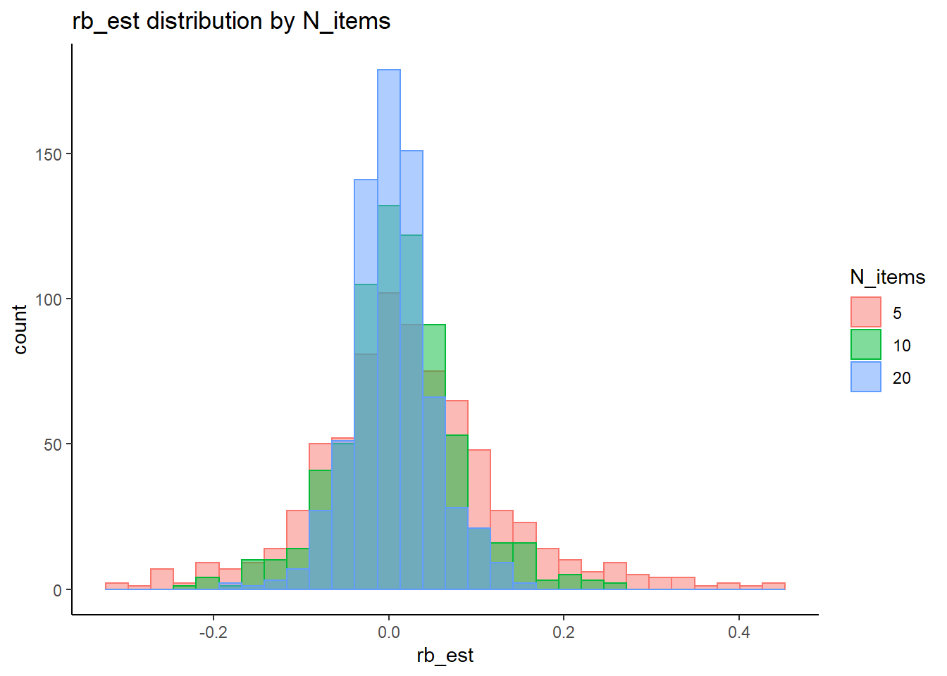
`stat_bin()` using `bins = 30`. Pick better value with `binwidth`.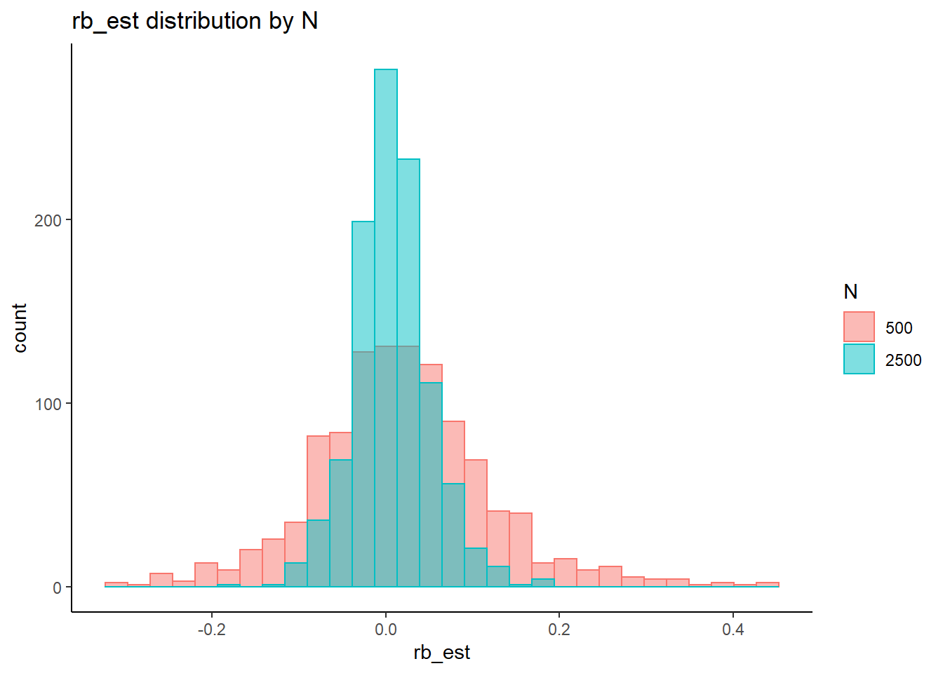
=============================
Tests of Homogeneity of Variance
Levenes Test: N_cat
Levene's Test for Homogeneity of Variance (center = "mean")
Df F value Pr(>F)
group 3 5.06 0.0017 **
2134
---
Signif. codes: 0 '***' 0.001 '**' 0.01 '*' 0.05 '.' 0.1 ' ' 1
Levenes Test: N_items
Levene's Test for Homogeneity of Variance (center = "mean")
Df F value Pr(>F)
group 2 129 <0.0000000000000002 ***
2135
---
Signif. codes: 0 '***' 0.001 '**' 0.01 '*' 0.05 '.' 0.1 ' ' 1
Levenes Test: N
Levene's Test for Homogeneity of Variance (center = "mean")
Df F value Pr(>F)
group 1 361 <0.0000000000000002 ***
2136
---
Signif. codes: 0 '***' 0.001 '**' 0.01 '*' 0.05 '.' 0.1 ' ' 1fit <- summary(aov(rb_est ~ N_cat*N_items*N, data=rb))
fit Df Sum Sq Mean Sq F value Pr(>F)
N_cat 3 0.06 0.0206 3.37 0.01781 *
N_items 2 0.14 0.0676 11.07 0.000016 ***
N 1 0.07 0.0739 12.10 0.00051 ***
N_cat:N_items 6 0.06 0.0100 1.64 0.13233
N_cat:N 3 0.03 0.0100 1.63 0.17972
N_items:N 2 0.04 0.0216 3.53 0.02952 *
N_cat:N_items:N 6 0.02 0.0027 0.43 0.85622
Residuals 2114 12.91 0.0061
---
Signif. codes: 0 '***' 0.001 '**' 0.01 '*' 0.05 '.' 0.1 ' ' 1eta_est <- (fit[[1]]$`Sum Sq`/sum(fit[[1]]$`Sum Sq`))[1:7]
cbind(omega2(fit),p_omega2(fit), eta_est) omega^2 partial-omega^2 eta_est
N_cat 0.0033 0.0033 0.00463
N_items 0.0092 0.0093 0.01015
N 0.0051 0.0052 0.00554
N_cat:N_items 0.0018 0.0018 0.00451
N_cat:N 0.0009 0.0009 0.00224
N_items:N 0.0023 0.0024 0.00323
N_cat:N_items:N -0.0016 -0.0016 0.00119saved_omega[5,] <- omega2(fit)
saved_eta[5,] <- eta_estResponse Time Factor Precision (\(\sigma_s\))
rb <- mydata %>%
filter(parameter_group == "sigma_s") %>%
group_by(condition, iter, N, N_cat, N_items) %>%
summarise(
rb_est = mean(post_median_bias_est)
)`summarise()` has grouped output by 'condition', 'iter', 'N', 'N_cat'. You can override using the `.groups` argument.## ANOVA on Relative Bias values
anova_assumptions_check(
dat = rb, outcome = 'rb_est',
factors = c('N_cat', 'N_items', 'N'),
model = as.formula('rb_est ~ N_cat*N_items*N'))
 =============================

 Tests and Plots of Normality: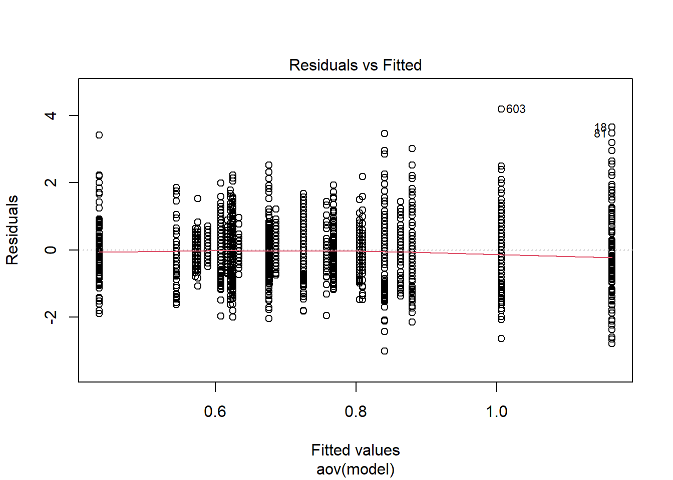
Shapiro-Wilks Test of Normality of Residuals:
Shapiro-Wilk normality test
data: res
W = 1, p-value <0.0000000000000002
K-S Test for Normality of Residuals:Warning in ks.test(aov.out$residuals, "pnorm", alternative = "two.sided"): ties
should not be present for the Kolmogorov-Smirnov test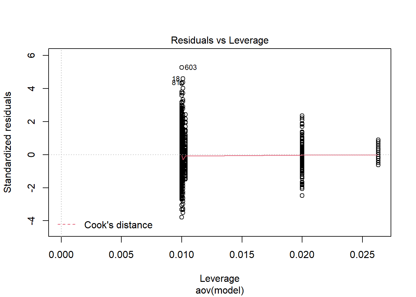
One-sample Kolmogorov-Smirnov test
data: aov.out$residuals
D = 0.1, p-value <0.0000000000000002
alternative hypothesis: two-sided`stat_bin()` using `bins = 30`. Pick better value with `binwidth`.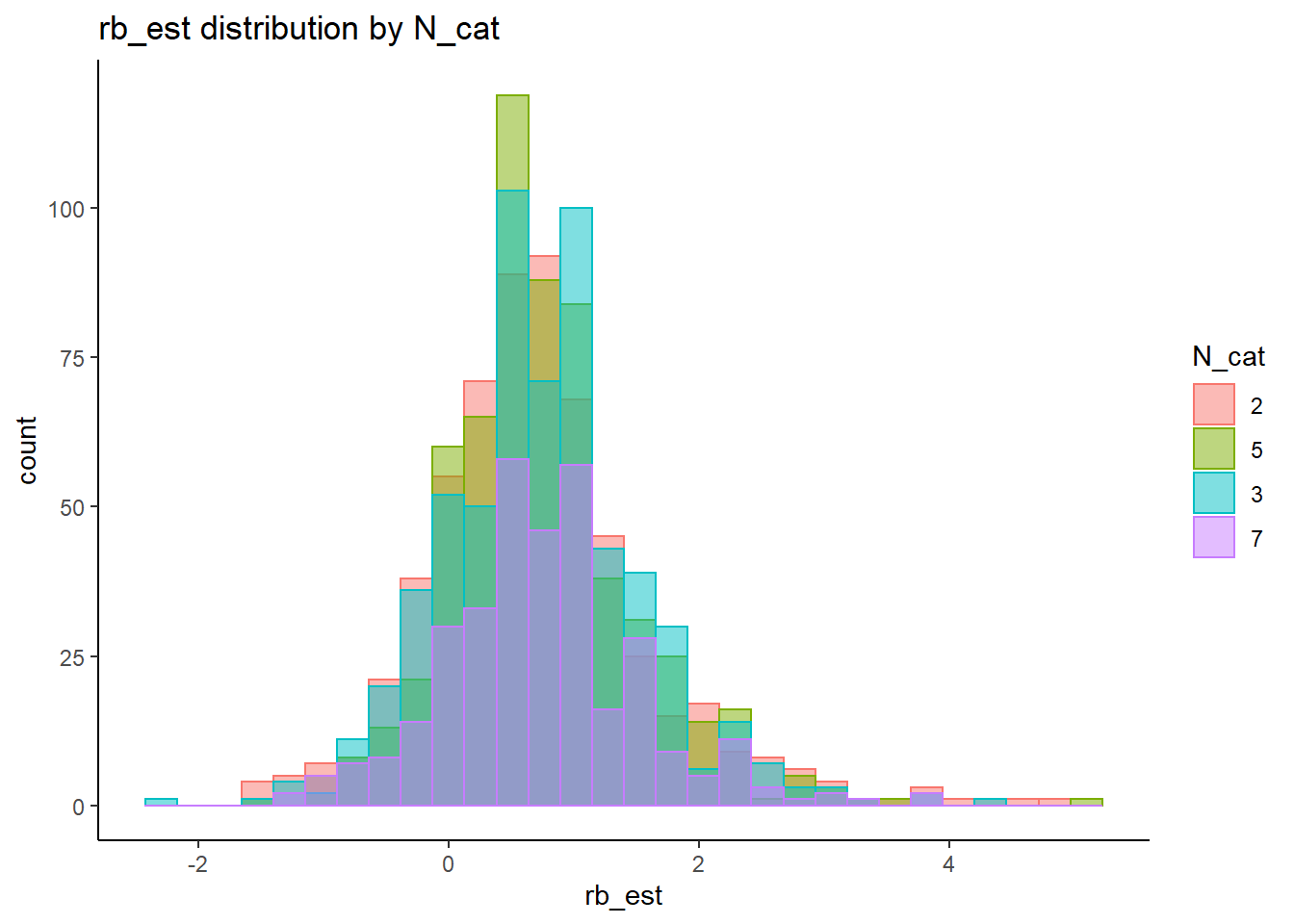
`stat_bin()` using `bins = 30`. Pick better value with `binwidth`.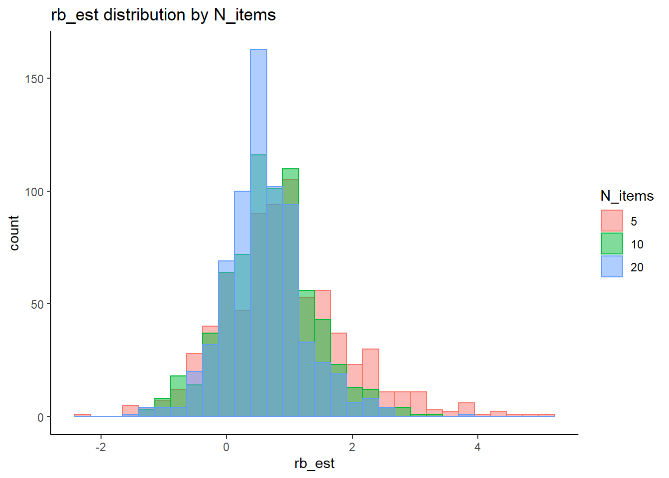
`stat_bin()` using `bins = 30`. Pick better value with `binwidth`.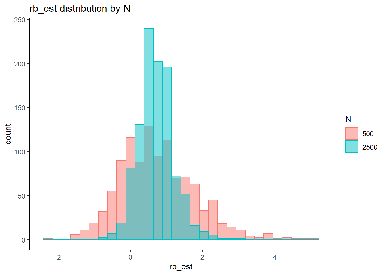
=============================
Tests of Homogeneity of Variance
Levenes Test: N_cat
Levene's Test for Homogeneity of Variance (center = "mean")
Df F value Pr(>F)
group 3 3.13 0.025 *
2130
---
Signif. codes: 0 '***' 0.001 '**' 0.01 '*' 0.05 '.' 0.1 ' ' 1
Levenes Test: N_items
Levene's Test for Homogeneity of Variance (center = "mean")
Df F value Pr(>F)
group 2 57.2 <0.0000000000000002 ***
2131
---
Signif. codes: 0 '***' 0.001 '**' 0.01 '*' 0.05 '.' 0.1 ' ' 1
Levenes Test: N
Levene's Test for Homogeneity of Variance (center = "mean")
Df F value Pr(>F)
group 1 406 <0.0000000000000002 ***
2132
---
Signif. codes: 0 '***' 0.001 '**' 0.01 '*' 0.05 '.' 0.1 ' ' 1fit <- summary(aov(rb_est ~ N_cat*N_items*N, data=rb))
fit Df Sum Sq Mean Sq F value Pr(>F)
N_cat 3 0 0.12 0.19 0.905
N_items 2 37 18.46 28.85 0.00000000000044 ***
N 1 1 0.76 1.19 0.275
N_cat:N_items 6 5 0.89 1.39 0.213
N_cat:N 3 2 0.63 0.98 0.400
N_items:N 2 5 2.44 3.82 0.022 *
N_cat:N_items:N 6 5 0.88 1.37 0.222
Residuals 2110 1350 0.64
---
Signif. codes: 0 '***' 0.001 '**' 0.01 '*' 0.05 '.' 0.1 ' ' 1eta_est <- (fit[[1]]$`Sum Sq`/sum(fit[[1]]$`Sum Sq`))[1:7]
cbind(omega2(fit),p_omega2(fit), eta_est) omega^2 partial-omega^2 eta_est
N_cat -0.0011 -0.0011 0.000257
N_items 0.0253 0.0254 0.026267
N 0.0001 0.0001 0.000544
N_cat:N_items 0.0011 0.0011 0.003807
N_cat:N 0.0000 0.0000 0.001342
N_items:N 0.0026 0.0026 0.003477
N_cat:N_items:N 0.0010 0.0010 0.003749saved_omega[6,] <- omega2(fit)
saved_eta[6,] <- eta_estFactor Covariance (\(\sigma_{st}\))
rb <- mydata %>%
filter(parameter_group == "sigma_st") %>%
group_by(condition, iter, N, N_cat, N_items) %>%
summarise(
rb_est = mean(post_median_bias_est)
)`summarise()` has grouped output by 'condition', 'iter', 'N', 'N_cat'. You can override using the `.groups` argument.## ANOVA on Relative Bias values
anova_assumptions_check(
dat = rb, outcome = 'rb_est',
factors = c('N_cat', 'N_items', 'N'),
model = as.formula('rb_est ~ N_cat*N_items*N'))
=============================
Tests and Plots of Normality: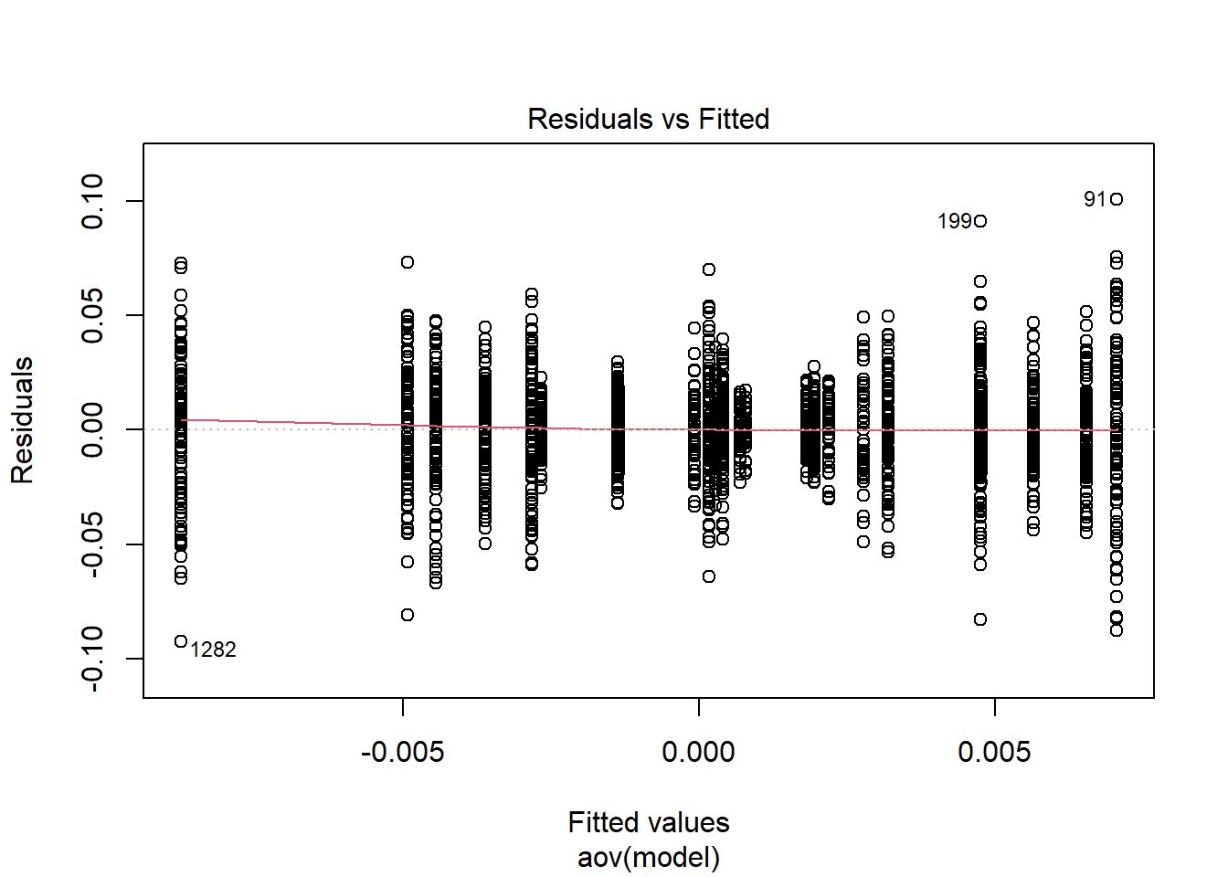
Shapiro-Wilks Test of Normality of Residuals:
Shapiro-Wilk normality test
data: res
W = 1, p-value <0.0000000000000002
K-S Test for Normality of Residuals:Warning in ks.test(aov.out$residuals, "pnorm", alternative = "two.sided"): ties
should not be present for the Kolmogorov-Smirnov test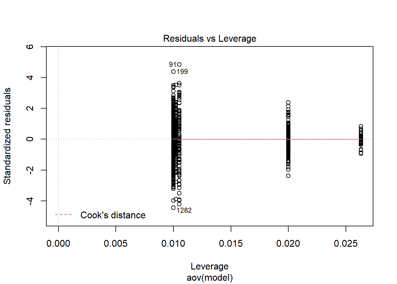
One-sample Kolmogorov-Smirnov test
data: aov.out$residuals
D = 0.5, p-value <0.0000000000000002
alternative hypothesis: two-sided`stat_bin()` using `bins = 30`. Pick better value with `binwidth`.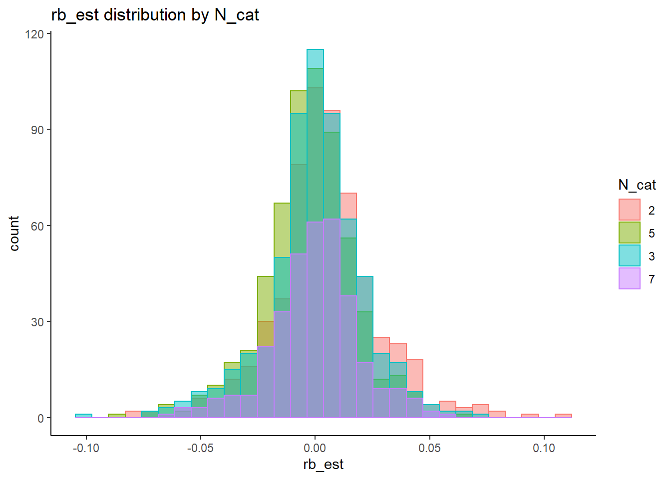
`stat_bin()` using `bins = 30`. Pick better value with `binwidth`.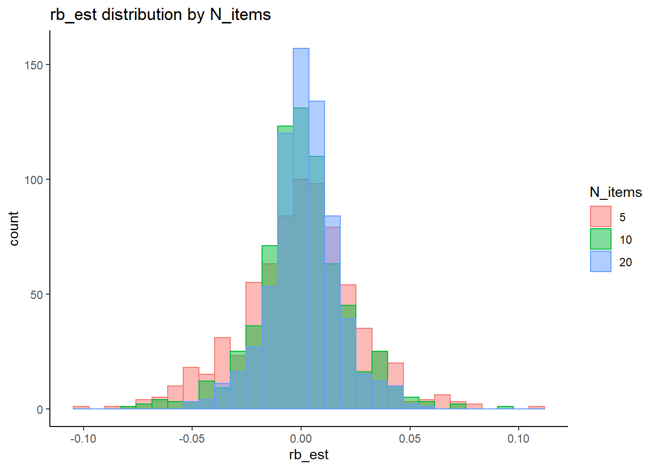
`stat_bin()` using `bins = 30`. Pick better value with `binwidth`.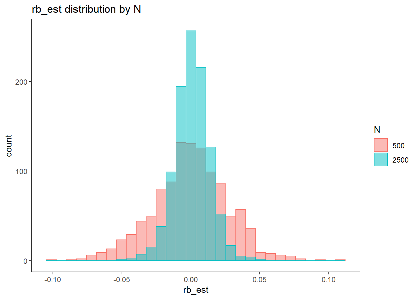
=============================
Tests of Homogeneity of Variance
Levenes Test: N_cat
Levene's Test for Homogeneity of Variance (center = "mean")
Df F value Pr(>F)
group 3 3.23 0.022 *
2125
---
Signif. codes: 0 '***' 0.001 '**' 0.01 '*' 0.05 '.' 0.1 ' ' 1
Levenes Test: N_items
Levene's Test for Homogeneity of Variance (center = "mean")
Df F value Pr(>F)
group 2 62.3 <0.0000000000000002 ***
2126
---
Signif. codes: 0 '***' 0.001 '**' 0.01 '*' 0.05 '.' 0.1 ' ' 1
Levenes Test: N
Levene's Test for Homogeneity of Variance (center = "mean")
Df F value Pr(>F)
group 1 371 <0.0000000000000002 ***
2127
---
Signif. codes: 0 '***' 0.001 '**' 0.01 '*' 0.05 '.' 0.1 ' ' 1fit <- summary(aov(rb_est ~ N_cat*N_items*N, data=rb))
fit Df Sum Sq Mean Sq F value Pr(>F)
N_cat 3 0.017 0.00581 13.25 0.000000014 ***
N_items 2 0.002 0.00088 2.00 0.136
N 1 0.001 0.00075 1.72 0.190
N_cat:N_items 6 0.007 0.00113 2.59 0.017 *
N_cat:N 3 0.001 0.00031 0.71 0.546
N_items:N 2 0.002 0.00114 2.61 0.074 .
N_cat:N_items:N 6 0.004 0.00067 1.52 0.166
Residuals 2105 0.922 0.00044
---
Signif. codes: 0 '***' 0.001 '**' 0.01 '*' 0.05 '.' 0.1 ' ' 1eta_est <- (fit[[1]]$`Sum Sq`/sum(fit[[1]]$`Sum Sq`))[1:7]
cbind(omega2(fit),p_omega2(fit), eta_est) omega^2 partial-omega^2 eta_est
N_cat 0.0168 0.0170 0.018218
N_items 0.0009 0.0009 0.001831
N 0.0003 0.0003 0.000788
N_cat:N_items 0.0044 0.0045 0.007112
N_cat:N -0.0004 -0.0004 0.000976
N_items:N 0.0015 0.0015 0.002393
N_cat:N_items:N 0.0014 0.0015 0.004192saved_omega[7,] <- omega2(fit)
saved_eta[7,] <- eta_estPID Relationship (\(\rho\))
rb <- mydata %>%
filter(parameter_group == "rho") %>%
group_by(condition, iter, N, N_cat, N_items) %>%
summarise(
rb_est = mean(post_median_bias_est)
)`summarise()` has grouped output by 'condition', 'iter', 'N', 'N_cat'. You can override using the `.groups` argument.## ANOVA on Relative Bias values
anova_assumptions_check(
dat = rb, outcome = 'rb_est',
factors = c('N_cat', 'N_items', 'N'),
model = as.formula('rb_est ~ N_cat*N_items*N'))
=============================
Tests and Plots of Normality: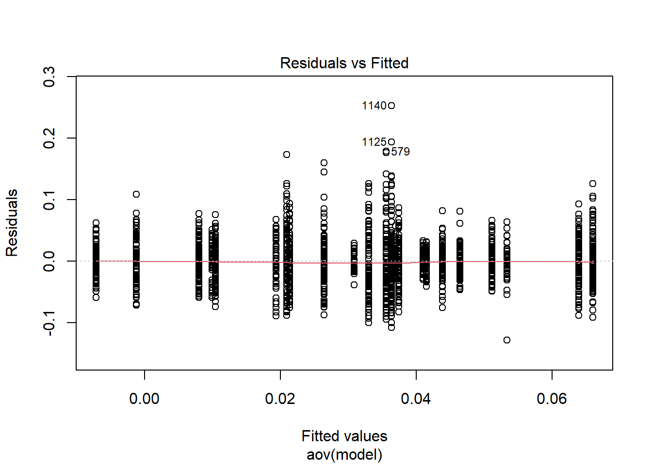
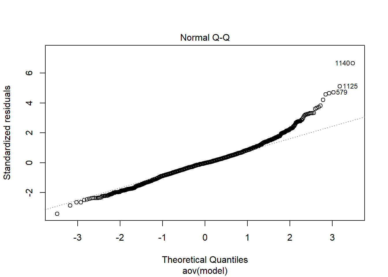
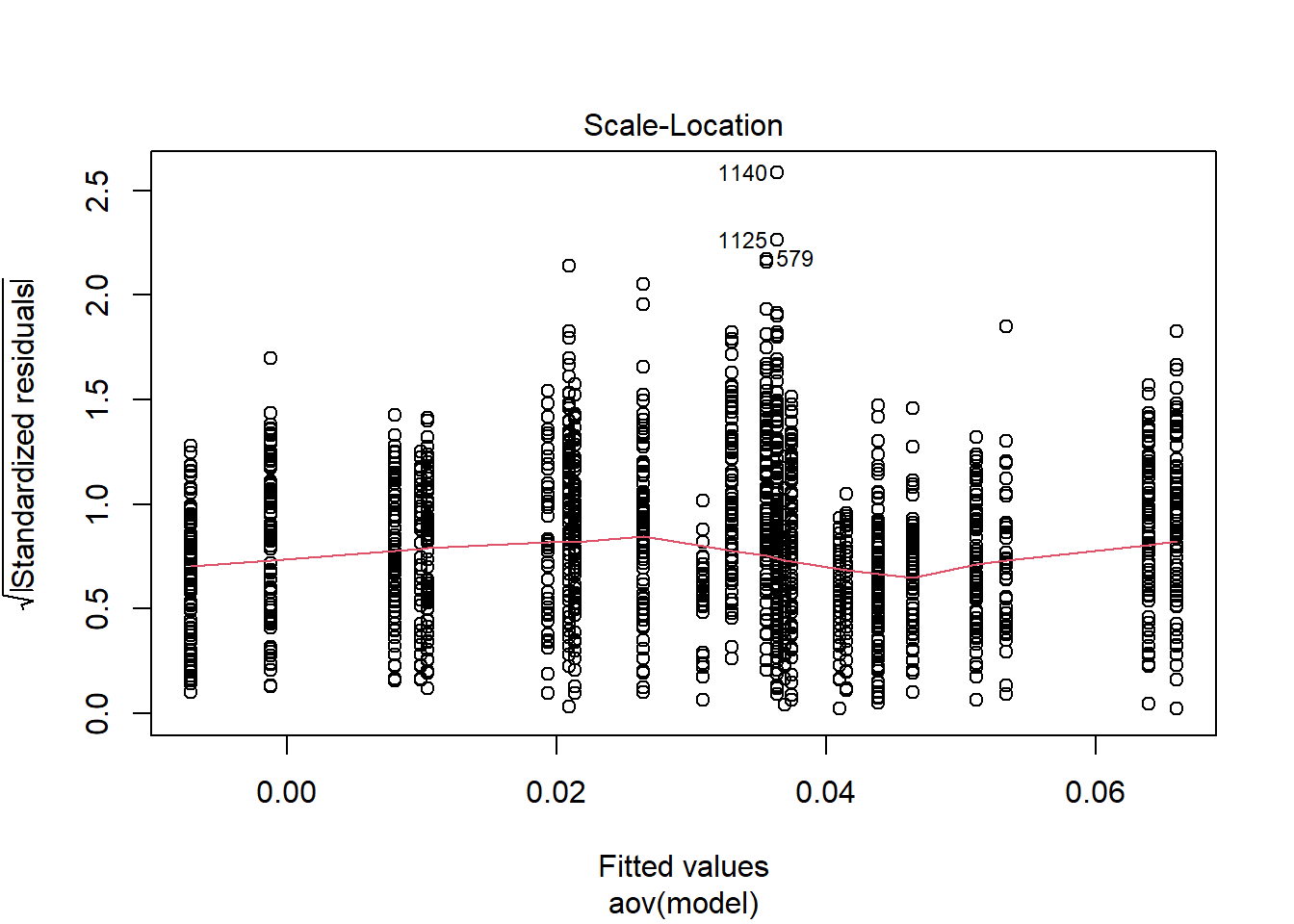
Shapiro-Wilks Test of Normality of Residuals:
Shapiro-Wilk normality test
data: res
W = 1, p-value <0.0000000000000002
K-S Test for Normality of Residuals:Warning in ks.test(aov.out$residuals, "pnorm", alternative = "two.sided"): ties
should not be present for the Kolmogorov-Smirnov test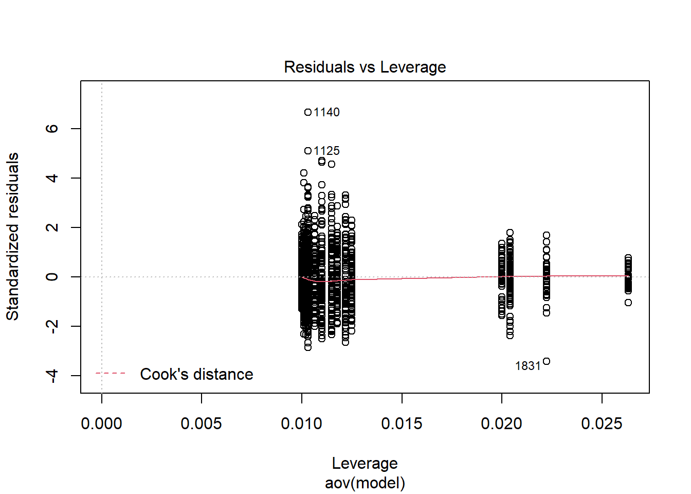
One-sample Kolmogorov-Smirnov test
data: aov.out$residuals
D = 0.5, p-value <0.0000000000000002
alternative hypothesis: two-sided`stat_bin()` using `bins = 30`. Pick better value with `binwidth`.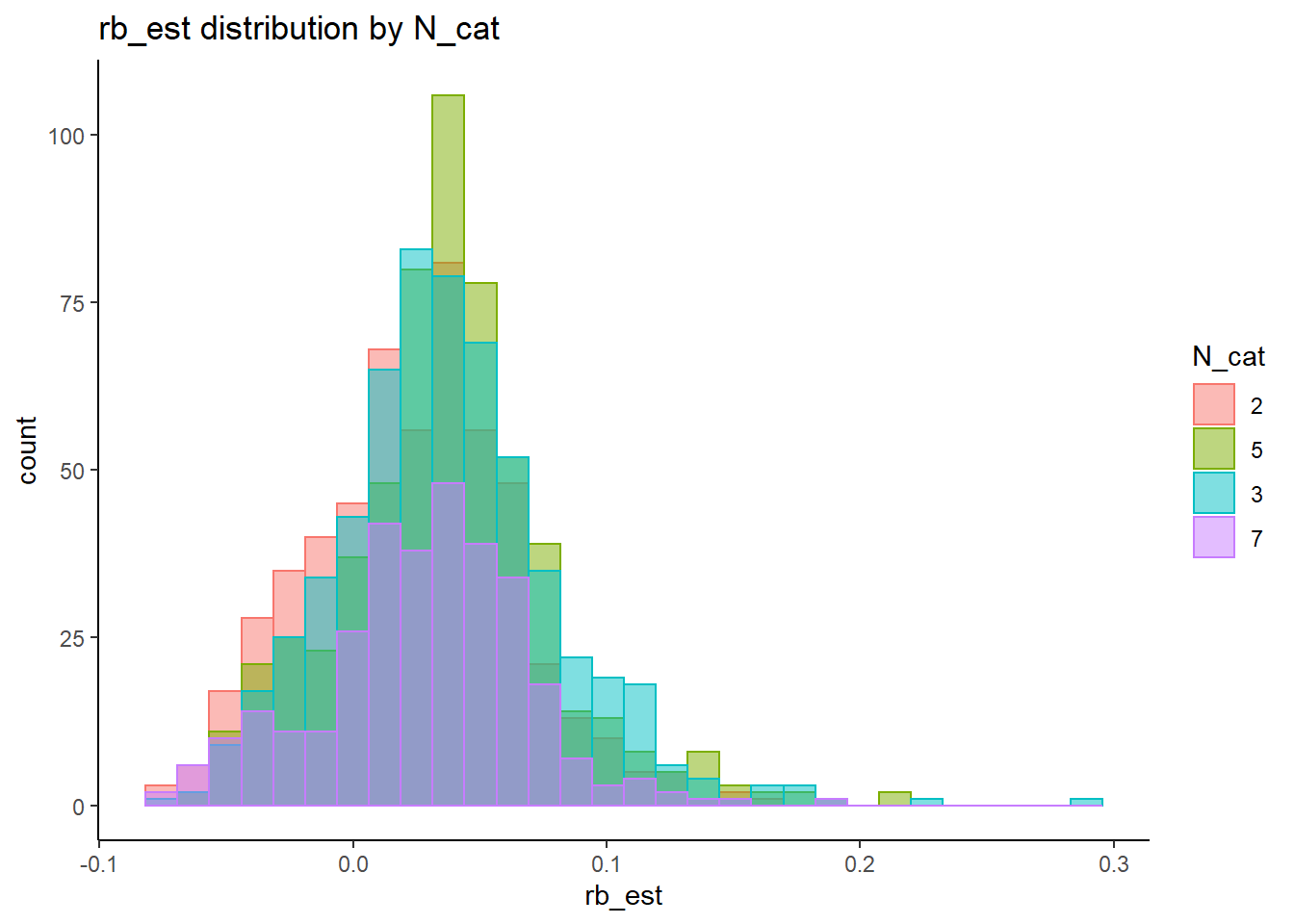
`stat_bin()` using `bins = 30`. Pick better value with `binwidth`.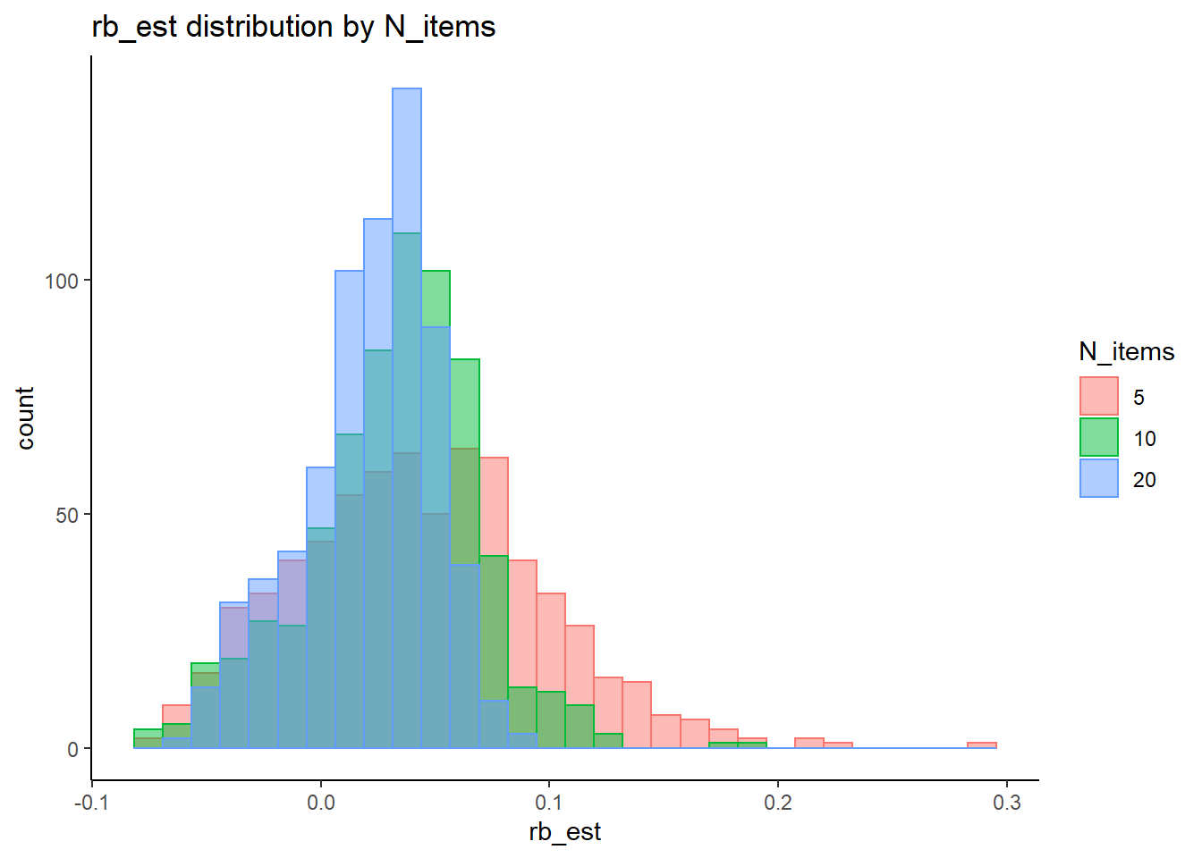
`stat_bin()` using `bins = 30`. Pick better value with `binwidth`.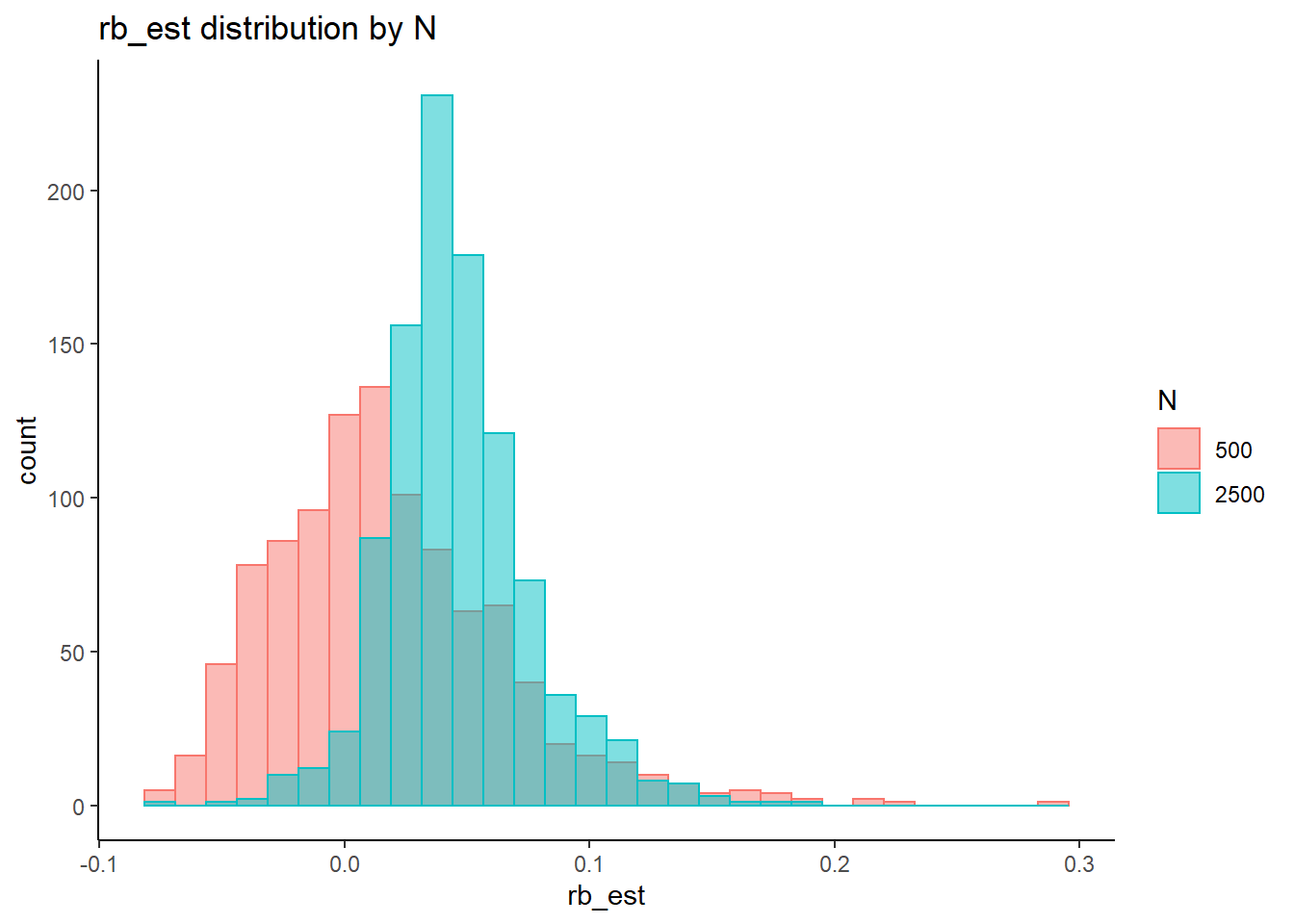
=============================
Tests of Homogeneity of Variance
Levenes Test: N_cat
Levene's Test for Homogeneity of Variance (center = "mean")
Df F value Pr(>F)
group 3 0.85 0.46
2028
Levenes Test: N_items
Levene's Test for Homogeneity of Variance (center = "mean")
Df F value Pr(>F)
group 2 113 <0.0000000000000002 ***
2029
---
Signif. codes: 0 '***' 0.001 '**' 0.01 '*' 0.05 '.' 0.1 ' ' 1
Levenes Test: N
Levene's Test for Homogeneity of Variance (center = "mean")
Df F value Pr(>F)
group 1 157 <0.0000000000000002 ***
2030
---
Signif. codes: 0 '***' 0.001 '**' 0.01 '*' 0.05 '.' 0.1 ' ' 1fit <- summary(aov(rb_est ~ N_cat*N_items*N, data=rb))
fit Df Sum Sq Mean Sq F value Pr(>F)
N_cat 3 0.073 0.024 16.70 0.0000000001 ***
N_items 2 0.172 0.086 59.44 < 0.0000000000000002 ***
N 1 0.420 0.420 289.99 < 0.0000000000000002 ***
N_cat:N_items 6 0.010 0.002 1.20 0.303
N_cat:N 3 0.003 0.001 0.64 0.592
N_items:N 2 0.007 0.003 2.32 0.098 .
N_cat:N_items:N 6 0.042 0.007 4.82 0.0000679088 ***
Residuals 2008 2.909 0.001
---
Signif. codes: 0 '***' 0.001 '**' 0.01 '*' 0.05 '.' 0.1 ' ' 1eta_est <- (fit[[1]]$`Sum Sq`/sum(fit[[1]]$`Sum Sq`))[1:7]
cbind(omega2(fit),p_omega2(fit), eta_est) omega^2 partial-omega^2 eta_est
N_cat 0.0188 0.0227 0.01997
N_items 0.0466 0.0544 0.04737
N 0.1151 0.1245 0.11555
N_cat:N_items 0.0005 0.0006 0.00287
N_cat:N -0.0004 -0.0005 0.00076
N_items:N 0.0011 0.0013 0.00185
N_cat:N_items:N 0.0091 0.0112 0.01153saved_omega[8,] <- omega2(fit)
saved_eta[8,] <- eta_estFactor Reliability (\(\omega\))
rb <- mydata %>%
filter(parameter_group == "omega") %>%
group_by(condition, iter, N, N_cat, N_items) %>%
summarise(
rb_est = mean(post_median_bias_est)
)`summarise()` has grouped output by 'condition', 'iter', 'N', 'N_cat'. You can override using the `.groups` argument.## ANOVA on Relative Bias values
anova_assumptions_check(
dat = rb, outcome = 'rb_est',
factors = c('N_cat', 'N_items', 'N'),
model = as.formula('rb_est ~ N_cat*N_items*N'))
=============================
Tests and Plots of Normality: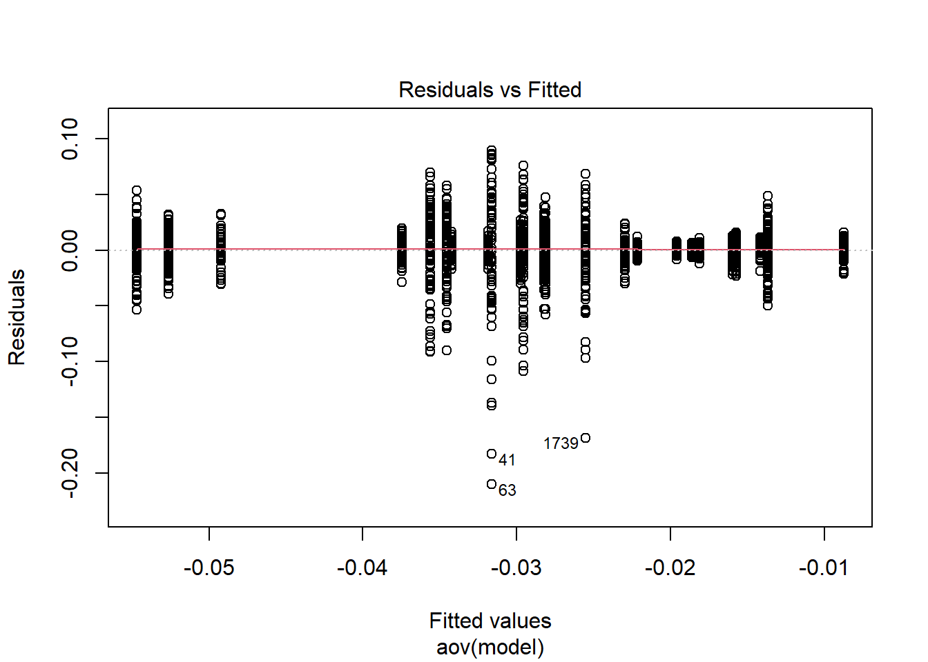
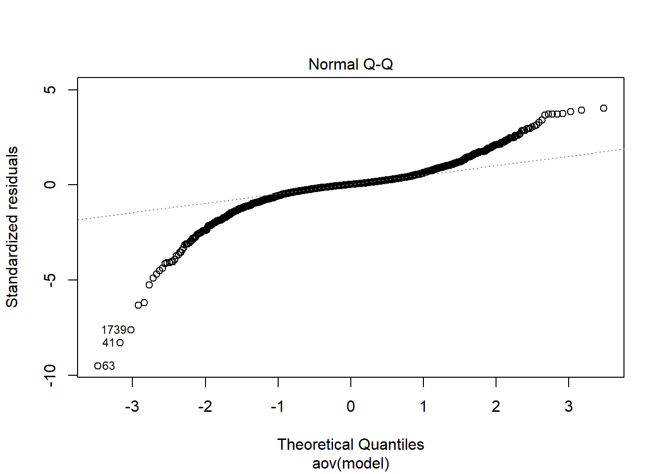
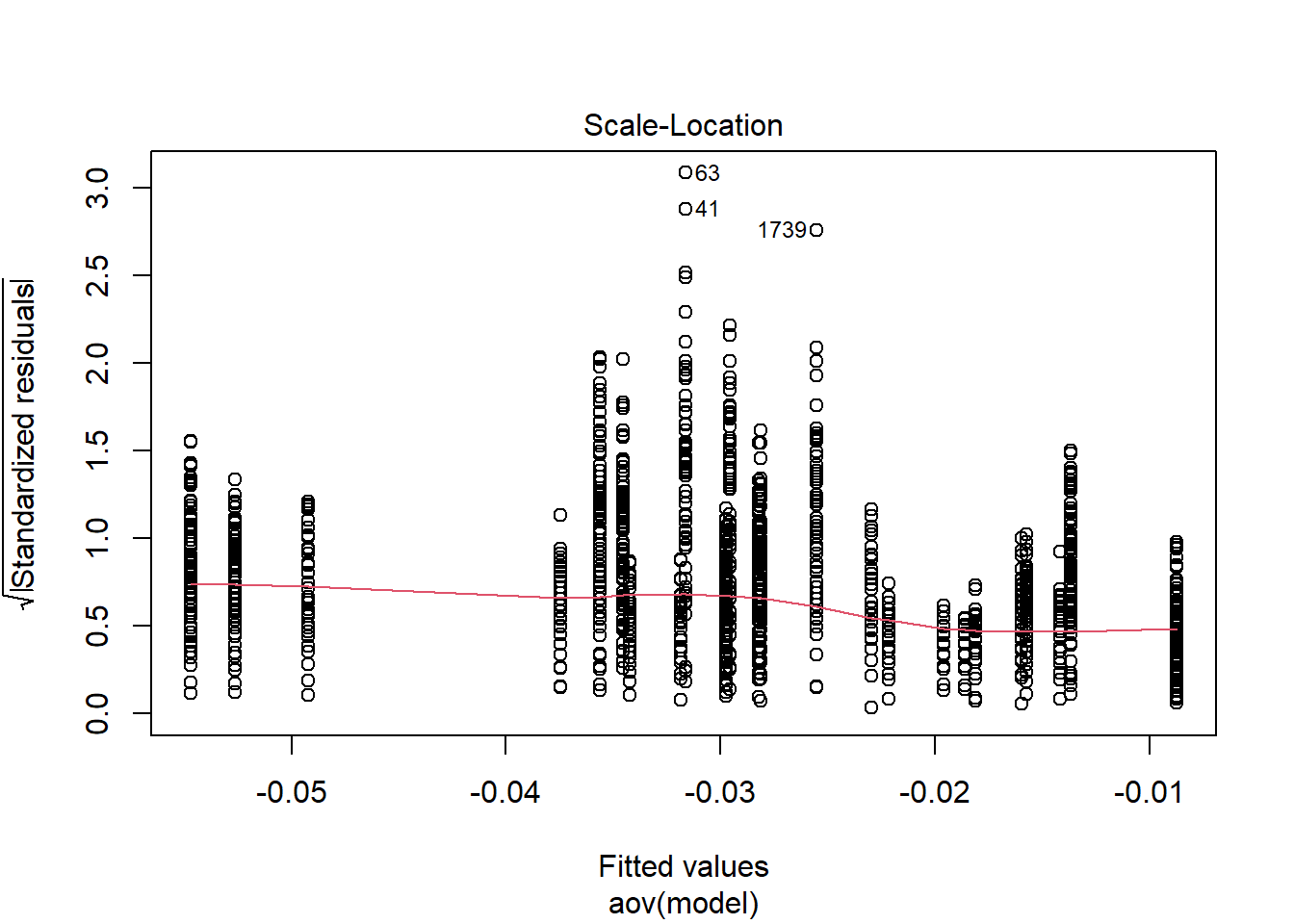
 Shapiro-Wilks Test of Normality of Residuals:

    Shapiro-Wilk normality test

data:  res
W = 0.8, p-value <0.0000000000000002


 K-S Test for Normality of Residuals:
Warning in ks.test(aov.out$residuals, "pnorm", alternative = "two.sided"): ties
should not be present for the Kolmogorov-Smirnov test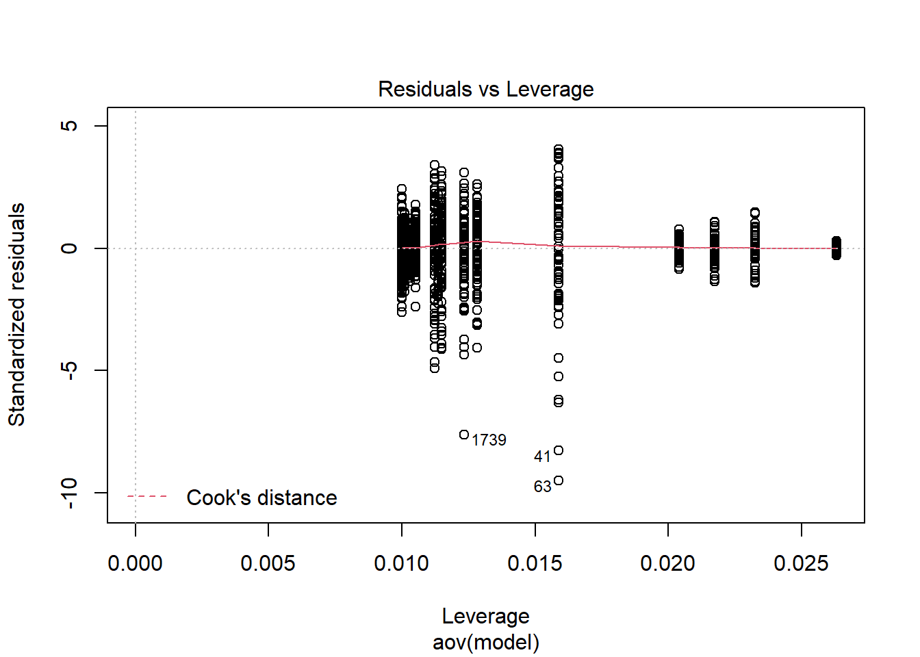
    One-sample Kolmogorov-Smirnov test

data:  aov.out$residuals
D = 0.5, p-value <0.0000000000000002
alternative hypothesis: two-sided
`stat_bin()` using `bins = 30`. Pick better value with `binwidth`.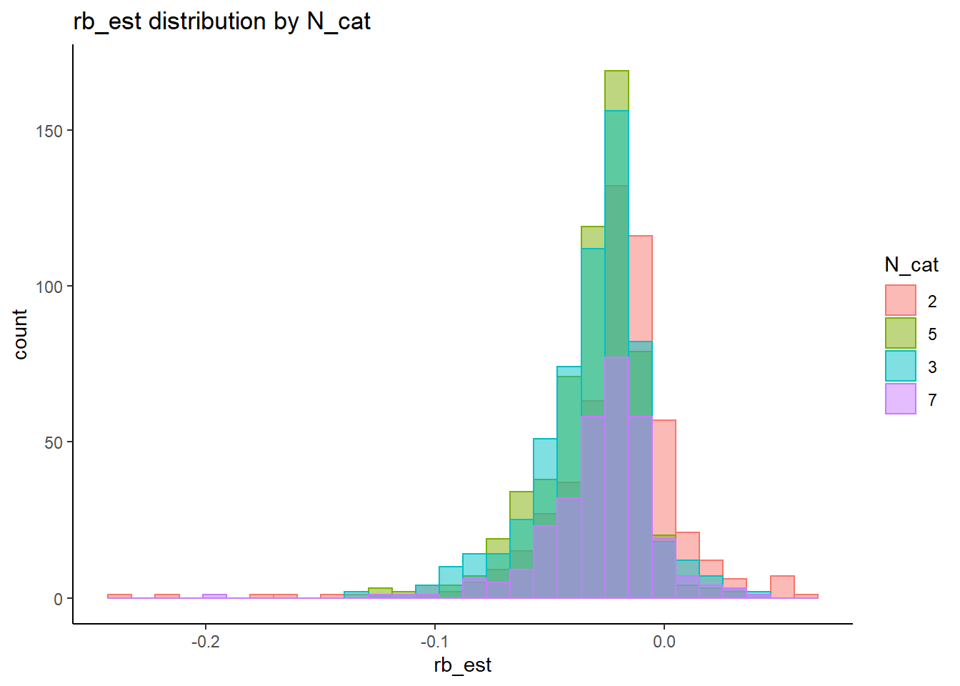
`stat_bin()` using `bins = 30`. Pick better value with `binwidth`.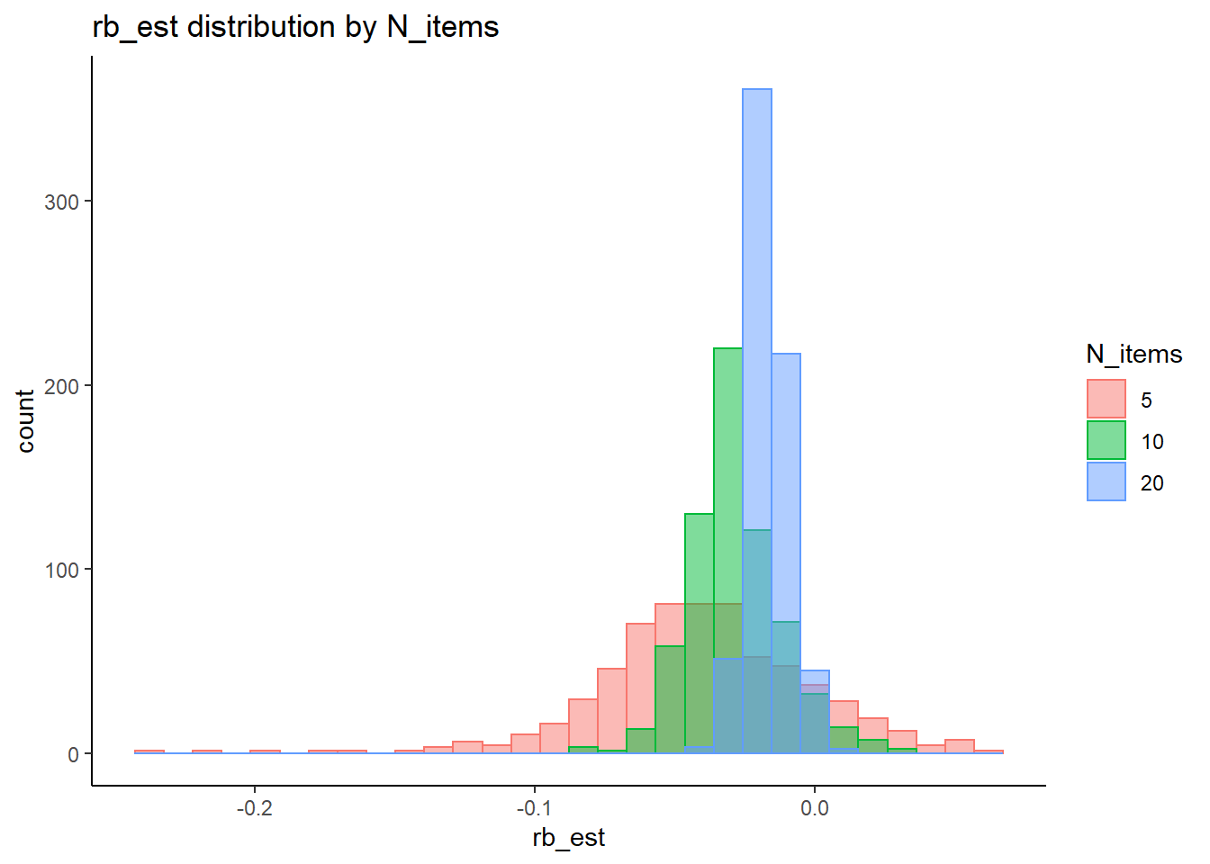
`stat_bin()` using `bins = 30`. Pick better value with `binwidth`.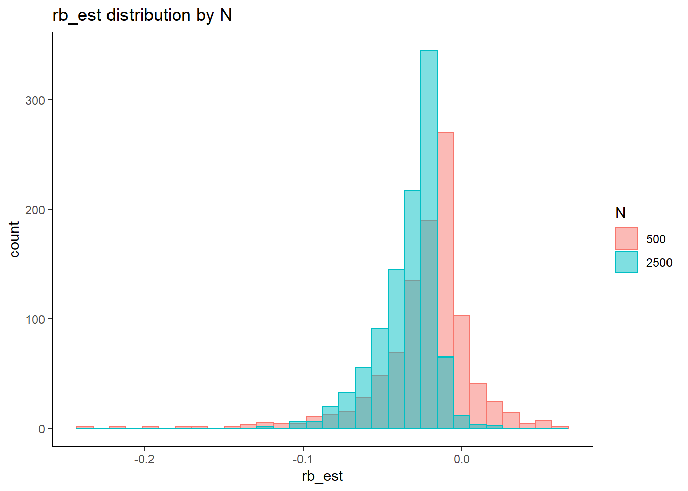
 =============================

 Tests of Homogeneity of Variance


 Levenes Test:  N_cat


Levene's Test for Homogeneity of Variance (center = "mean")
        Df F value Pr(>F)
group    3    3.36  0.018 *
      1987
---
Signif. codes:  0 '***' 0.001 '**' 0.01 '*' 0.05 '.' 0.1 ' ' 1


 Levenes Test:  N_items


Levene's Test for Homogeneity of Variance (center = "mean")
        Df F value              Pr(>F)
group    2     363 <0.0000000000000002 ***
      1988
---
Signif. codes:  0 '***' 0.001 '**' 0.01 '*' 0.05 '.' 0.1 ' ' 1


 Levenes Test:  N


Levene's Test for Homogeneity of Variance (center = "mean")
        Df F value        Pr(>F)
group    1      42 0.00000000011 ***
      1989
---
Signif. codes:  0 '***' 0.001 '**' 0.01 '*' 0.05 '.' 0.1 ' ' 1
fit <- summary(aov(rb_est ~ N_cat*N_items*N, data=rb))
fit Df Sum Sq Mean Sq F value Pr(>F)
N_cat 3 0.032 0.0105 21.23 0.00000000000016 ***
N_items 2 0.168 0.0842 169.56 < 0.0000000000000002 ***
N 1 0.062 0.0624 125.66 < 0.0000000000000002 ***
N_cat:N_items 6 0.004 0.0007 1.41 0.20634
N_cat:N 3 0.002 0.0007 1.38 0.24816
N_items:N 2 0.010 0.0052 10.43 0.00003113242259 ***
N_cat:N_items:N 6 0.013 0.0021 4.32 0.00024 ***
Residuals 1967 0.977 0.0005
---
Signif. codes: 0 '***' 0.001 '**' 0.01 '*' 0.05 '.' 0.1 ' ' 1eta_est <- (fit[[1]]$`Sum Sq`/sum(fit[[1]]$`Sum Sq`))[1:7]
cbind(omega2(fit),p_omega2(fit), eta_est) omega^2 partial-omega^2 eta_est
N_cat 0.0237 0.0296 0.02493
N_items 0.1319 0.1448 0.13274
N 0.0488 0.0589 0.04918
N_cat:N_items 0.0010 0.0012 0.00331
N_cat:N 0.0004 0.0006 0.00162
N_items:N 0.0074 0.0094 0.00817
N_cat:N_items:N 0.0078 0.0099 0.01015saved_omega[9,] <- omega2(fit)
saved_eta[9,] <- eta_estManuscript Figures and Tables (latex formated)
Tables
keep_cols <- c("condition", "iter", "N", "N_items", "N_cat", "parameter_group", "post_median_rb_est", "post_median_bias_est")

tbl_dat <- mydata %>%
  select(all_of(keep_cols)) %>%
  filter(
    !is.na(parameter_group)
    , parameter_group != "lambda (STD)"
  )

# get average Rhat and SD for each condition and parameter group
sum_tab <- tbl_dat %>%
  group_by(N_cat, N_items, N, parameter_group) %>%
  summarise(
    Post_Median_RB_Mean = mean(post_median_rb_est),
    Post_Median_AB_Mean = mean(post_median_bias_est)
  )
`summarise()` has grouped output by 'N_cat', 'N_items', 'N'. You can override using the `.groups` argument.# table 1: 2 category data
T1 <- sum_tab %>%
filter(N_cat == 2) %>%
pivot_wider(
id_cols = c("parameter_group", "N")
, names_from = "N_items"
, values_from = all_of(c("Post_Median_RB_Mean", "Post_Median_AB_Mean"))
) %>%
arrange(.,parameter_group)
# reordering of rows to more logical for presentation
#T1 <- T1[c(3:4, 15:18, 1:2, 5:8, 13:14, 11:12, 9:10) ,]
print(
xtable(
T1[c(3:4, 15:18, 1:2, 5:8, 13:14, 11:12, 9:10) , ]
, caption = c("Posterior Bias: Dichotomous items")
,align = "lllrrrrrr"
),
include.rownames=F,
booktabs=T
)% latex table generated in R 4.0.5 by xtable 1.8-4 package
% Sun Feb 13 15:23:00 2022
\begin{table}[ht]
\centering
\begin{tabular}{llrrrrrr}
\toprule
parameter\_group & N & Post\_Median\_RB\_Mean\_5 & Post\_Median\_RB\_Mean\_10 & Post\_Median\_RB\_Mean\_20 & Post\_Median\_AB\_Mean\_5 & Post\_Median\_AB\_Mean\_10 & Post\_Median\_AB\_Mean\_20 \\
\midrule
lambda & 500 & -25.57 & -13.95 & -10.25 & -0.23 & -0.13 & -0.09 \\
lambda & 2500 & -16.49 & -13.87 & -13.83 & -0.15 & -0.12 & -0.12 \\
tau & 500 & -8.28 & -2.85 & 6.40 & -0.00 & 0.01 & -0.01 \\
tau & 2500 & -2.28 & -3.30 & -15.94 & -0.00 & -0.00 & -0.00 \\
theta & 500 & -9.86 & -5.68 & -4.72 & -0.18 & -0.10 & -0.09 \\
theta & 2500 & -11.40 & -10.66 & -10.84 & -0.21 & -0.19 & -0.20 \\
beta\_lrt & 500 & 0.09 & -1.07 & -1.31 & 0.00 & -0.02 & -0.02 \\
beta\_lrt & 2500 & 0.55 & 0.56 & 0.30 & 0.01 & 0.01 & 0.00 \\
sigma\_lrt & 500 & 1.29 & 0.66 & 0.17 & 0.05 & 0.03 & 0.01 \\
sigma\_lrt & 2500 & 0.42 & 0.14 & 0.08 & 0.02 & 0.01 & 0.00 \\
sigma\_s & 500 & 11.64 & 6.25 & 4.35 & 1.16 & 0.63 & 0.44 \\
sigma\_s & 2500 & 7.68 & 6.77 & 5.76 & 0.77 & 0.68 & 0.58 \\
sigma\_st & 500 & -9.70 & -6.54 & -4.40 & 0.01 & 0.00 & 0.00 \\
sigma\_st & 2500 & -7.76 & -2.67 & -6.57 & 0.01 & 0.00 & 0.00 \\
rho & 500 & 33.04 & -1.20 & -7.13 & 0.03 & -0.00 & -0.01 \\
rho & 2500 & 37.40 & 43.85 & 36.33 & 0.04 & 0.04 & 0.04 \\
omega & 500 & -3.94 & -1.53 & -0.93 & -0.03 & -0.01 & -0.01 \\
omega & 2500 & -4.31 & -3.34 & -1.92 & -0.03 & -0.03 & -0.02 \\
\bottomrule
\end{tabular}
\caption{Posterior Bias: Dichotomous items}
\end{table}# table 2: 5 category data
T2 <- sum_tab %>%
filter(N_cat == 5) %>%
pivot_wider(
id_cols = c("parameter_group", "N")
, names_from = "N_items"
, values_from = all_of(c("Post_Median_RB_Mean", "Post_Median_AB_Mean"))
) %>%
arrange(.,parameter_group)
# reordering of rows to more logical for presentation
print(
xtable(
T2[c(3:4, 15:18, 1:2, 5:8, 13:14, 11:12, 9:10) , ]
, caption = c("Posterior Bias: Five category items")
,align = "lllrrrrrr"
),
include.rownames=F,
booktabs=T
)% latex table generated in R 4.0.5 by xtable 1.8-4 package
% Sun Feb 13 15:23:00 2022
\begin{table}[ht]
\centering
\begin{tabular}{llrrrrrr}
\toprule
parameter\_group & N & Post\_Median\_RB\_Mean\_5 & Post\_Median\_RB\_Mean\_10 & Post\_Median\_RB\_Mean\_20 & Post\_Median\_AB\_Mean\_5 & Post\_Median\_AB\_Mean\_10 & Post\_Median\_AB\_Mean\_20 \\
\midrule
lambda & 500 & -14.66 & -13.48 & -12.76 & -0.13 & -0.12 & -0.11 \\
lambda & 2500 & -14.93 & -14.61 & -14.40 & -0.13 & -0.13 & -0.13 \\
tau & 500 & -3.81 & -6.67 & -22.63 & 0.00 & -0.00 & 0.01 \\
tau & 2500 & -8.11 & -9.11 & -16.54 & -0.02 & -0.01 & -0.01 \\
theta & 500 & -9.39 & -9.83 & -9.50 & -0.17 & -0.18 & -0.17 \\
theta & 2500 & -11.81 & -11.84 & -11.76 & -0.21 & -0.21 & -0.21 \\
beta\_lrt & 500 & 0.53 & -0.30 & -0.82 & 0.01 & -0.00 & -0.01 \\
beta\_lrt & 2500 & 1.42 & 0.57 & 0.39 & 0.02 & 0.01 & 0.01 \\
sigma\_lrt & 500 & 1.00 & 0.33 & 0.31 & 0.04 & 0.01 & 0.01 \\
sigma\_lrt & 2500 & 0.15 & 0.08 & 0.13 & 0.01 & 0.00 & 0.01 \\
sigma\_s & 500 & 10.07 & 7.25 & 6.22 & 1.01 & 0.73 & 0.62 \\
sigma\_s & 2500 & 8.09 & 6.86 & 5.71 & 0.81 & 0.69 & 0.57 \\
sigma\_st & 500 & -6.78 & -6.13 & -4.97 & -0.00 & -0.00 & -0.00 \\
sigma\_st & 2500 & -1.90 & -3.69 & -1.87 & -0.00 & -0.00 & -0.00 \\
rho & 500 & 35.60 & 21.37 & 10.46 & 0.04 & 0.02 & 0.01 \\
rho & 2500 & 65.98 & 46.40 & 40.98 & 0.07 & 0.05 & 0.04 \\
omega & 500 & -4.44 & -3.17 & -1.69 & -0.04 & -0.03 & -0.02 \\
omega & 2500 & -6.57 & -3.85 & -2.08 & -0.05 & -0.03 & -0.02 \\
\bottomrule
\end{tabular}
\caption{Posterior Bias: Five category items}
\end{table}# table 3: 3 category data
T3 <- sum_tab %>%
filter(N_cat == 3) %>%
pivot_wider(
id_cols = c("parameter_group", "N")
, names_from = "N_items"
, values_from = all_of(c("Post_Median_RB_Mean", "Post_Median_AB_Mean"))
) %>%
arrange(.,parameter_group)
# reordering of rows to more logical for presentation
print(
xtable(
T3[c(3:4, 15:18, 1:2, 5:8, 13:14, 11:12, 9:10) , ]
, caption = c("Posterior Bias: three category items")
,align = "lllrrrrrr"
),
include.rownames=F,
booktabs=T
)% latex table generated in R 4.0.5 by xtable 1.8-4 package
% Sun Feb 13 15:23:00 2022
\begin{table}[ht]
\centering
\begin{tabular}{llrrrrrr}
\toprule
parameter\_group & N & Post\_Median\_RB\_Mean\_5 & Post\_Median\_RB\_Mean\_10 & Post\_Median\_RB\_Mean\_20 & Post\_Median\_AB\_Mean\_5 & Post\_Median\_AB\_Mean\_10 & Post\_Median\_AB\_Mean\_20 \\
\midrule
lambda & 500 & -14.18 & -13.31 & -12.47 & -0.13 & -0.12 & -0.11 \\
lambda & 2500 & -15.38 & -15.69 & -15.88 & -0.14 & -0.14 & -0.14 \\
tau & 500 & 58.04 & -50.96 & -67.29 & 0.12 & 0.11 & 0.11 \\
tau & 2500 & 54.39 & -48.43 & -52.75 & 0.12 & 0.11 & 0.11 \\
theta & 500 & -7.28 & -8.71 & -8.87 & -0.13 & -0.16 & -0.16 \\
theta & 2500 & -11.89 & -12.49 & -12.77 & -0.22 & -0.23 & -0.23 \\
beta\_lrt & 500 & 0.35 & 0.05 & -0.78 & 0.01 & 0.00 & -0.01 \\
beta\_lrt & 2500 & 1.43 & 0.75 & 0.06 & 0.02 & 0.01 & 0.00 \\
sigma\_lrt & 500 & 0.96 & 0.27 & 0.08 & 0.04 & 0.01 & 0.00 \\
sigma\_lrt & 2500 & 0.51 & 0.21 & 0.12 & 0.02 & 0.01 & 0.00 \\
sigma\_s & 500 & 8.40 & 6.76 & 6.08 & 0.84 & 0.68 & 0.61 \\
sigma\_s & 2500 & 8.63 & 8.05 & 6.18 & 0.86 & 0.81 & 0.62 \\
sigma\_st & 500 & -12.05 & 0.22 & 9.01 & -0.01 & 0.00 & 0.01 \\
sigma\_st & 2500 & 0.55 & 0.38 & 2.51 & 0.00 & 0.00 & 0.00 \\
rho & 500 & 36.35 & 26.41 & 8.04 & 0.04 & 0.03 & 0.01 \\
rho & 2500 & 63.92 & 51.16 & 36.93 & 0.06 & 0.05 & 0.04 \\
omega & 500 & -3.69 & -3.16 & -1.67 & -0.03 & -0.03 & -0.02 \\
omega & 2500 & -6.82 & -4.21 & -2.35 & -0.05 & -0.04 & -0.02 \\
\bottomrule
\end{tabular}
\caption{Posterior Bias: three category items}
\end{table}# table 4: 7 category data
T4 <- sum_tab %>%
filter(N_cat == 5) %>%
pivot_wider(
id_cols = c("parameter_group", "N")
, names_from = "N_items"
, values_from = all_of(c("Post_Median_RB_Mean", "Post_Median_AB_Mean"))
) %>%
arrange(.,parameter_group)
# reordering of rows to more logical for presentation
print(
xtable(
T4[c(3:4, 15:18, 1:2, 5:8, 13:14, 11:12, 9:10) , ]
, caption = c("Posterior Bias: seven category items")
,align = "lllrrrrrr"
),
include.rownames=F,
booktabs=T
)% latex table generated in R 4.0.5 by xtable 1.8-4 package
% Sun Feb 13 15:23:00 2022
\begin{table}[ht]
\centering
\begin{tabular}{llrrrrrr}
\toprule
parameter\_group & N & Post\_Median\_RB\_Mean\_5 & Post\_Median\_RB\_Mean\_10 & Post\_Median\_RB\_Mean\_20 & Post\_Median\_AB\_Mean\_5 & Post\_Median\_AB\_Mean\_10 & Post\_Median\_AB\_Mean\_20 \\
\midrule
lambda & 500 & -14.66 & -13.48 & -12.76 & -0.13 & -0.12 & -0.11 \\
lambda & 2500 & -14.93 & -14.61 & -14.40 & -0.13 & -0.13 & -0.13 \\
tau & 500 & -3.81 & -6.67 & -22.63 & 0.00 & -0.00 & 0.01 \\
tau & 2500 & -8.11 & -9.11 & -16.54 & -0.02 & -0.01 & -0.01 \\
theta & 500 & -9.39 & -9.83 & -9.50 & -0.17 & -0.18 & -0.17 \\
theta & 2500 & -11.81 & -11.84 & -11.76 & -0.21 & -0.21 & -0.21 \\
beta\_lrt & 500 & 0.53 & -0.30 & -0.82 & 0.01 & -0.00 & -0.01 \\
beta\_lrt & 2500 & 1.42 & 0.57 & 0.39 & 0.02 & 0.01 & 0.01 \\
sigma\_lrt & 500 & 1.00 & 0.33 & 0.31 & 0.04 & 0.01 & 0.01 \\
sigma\_lrt & 2500 & 0.15 & 0.08 & 0.13 & 0.01 & 0.00 & 0.01 \\
sigma\_s & 500 & 10.07 & 7.25 & 6.22 & 1.01 & 0.73 & 0.62 \\
sigma\_s & 2500 & 8.09 & 6.86 & 5.71 & 0.81 & 0.69 & 0.57 \\
sigma\_st & 500 & -6.78 & -6.13 & -4.97 & -0.00 & -0.00 & -0.00 \\
sigma\_st & 2500 & -1.90 & -3.69 & -1.87 & -0.00 & -0.00 & -0.00 \\
rho & 500 & 35.60 & 21.37 & 10.46 & 0.04 & 0.02 & 0.01 \\
rho & 2500 & 65.98 & 46.40 & 40.98 & 0.07 & 0.05 & 0.04 \\
omega & 500 & -4.44 & -3.17 & -1.69 & -0.04 & -0.03 & -0.02 \\
omega & 2500 & -6.57 & -3.85 & -2.08 & -0.05 & -0.03 & -0.02 \\
\bottomrule
\end{tabular}
\caption{Posterior Bias: seven category items}
\end{table}# effect size
print(
xtable(
t(saved_eta)
, caption = c("Effect of design factors on relative bias estimates: eta2")
,align = "lrrrrrrrrr", digits = 3
),
include.rownames=T,
booktabs=T
)% latex table generated in R 4.0.5 by xtable 1.8-4 package
% Sun Feb 13 15:23:00 2022
\begin{table}[ht]
\centering
\begin{tabular}{lrrrrrrrrr}
\toprule
& lambda & tau & theta & beta\_lrt & sigma\_lrt & sigma\_s & sigma\_ts & rho & omega \\
\midrule
N\_cat & 0.015 & 0.563 & 0.006 & 0.010 & 0.005 & 0.000 & 0.018 & 0.020 & 0.025 \\
N\_items & 0.031 & 0.000 & 0.003 & 0.051 & 0.010 & 0.026 & 0.002 & 0.047 & 0.133 \\
N & 0.001 & 0.006 & 0.035 & 0.065 & 0.006 & 0.001 & 0.001 & 0.116 & 0.049 \\
N\_cat:N\_items & 0.039 & 0.003 & 0.011 & 0.003 & 0.005 & 0.004 & 0.007 & 0.003 & 0.003 \\
N\_cat:N & 0.008 & 0.005 & 0.003 & 0.002 & 0.002 & 0.001 & 0.001 & 0.001 & 0.002 \\
N\_items:N & 0.014 & 0.000 & 0.002 & 0.001 & 0.003 & 0.003 & 0.002 & 0.002 & 0.008 \\
N\_cat:N\_items:N & 0.012 & 0.001 & 0.004 & 0.005 & 0.001 & 0.004 & 0.004 & 0.012 & 0.010 \\
\bottomrule
\end{tabular}
\caption{Effect of design factors on relative bias estimates: eta2}
\end{table}print(
xtable(
t(saved_omega)
, caption = c("Effect of design factors on relative bias estimates: omega2")
,align = "lrrrrrrrrr", digits = 3
),
include.rownames=T,
booktabs=T
)% latex table generated in R 4.0.5 by xtable 1.8-4 package
% Sun Feb 13 15:23:00 2022
\begin{table}[ht]
\centering
\begin{tabular}{lrrrrrrrrr}
\toprule
& lambda & tau & theta & beta\_lrt & sigma\_lrt & sigma\_s & sigma\_ts & rho & omega \\
\midrule
N\_cat & 0.014 & 0.562 & 0.005 & 0.009 & 0.003 & -0.001 & 0.017 & 0.019 & 0.024 \\
N\_items & 0.030 & -0.000 & 0.002 & 0.050 & 0.009 & 0.025 & 0.001 & 0.047 & 0.132 \\
N & 0.000 & 0.006 & 0.034 & 0.064 & 0.005 & 0.000 & 0.000 & 0.115 & 0.049 \\
N\_cat:N\_items & 0.036 & 0.002 & 0.008 & 0.000 & 0.002 & 0.001 & 0.004 & 0.000 & 0.001 \\
N\_cat:N & 0.007 & 0.004 & 0.001 & 0.001 & 0.001 & -0.000 & -0.000 & -0.000 & 0.000 \\
N\_items:N & 0.013 & -0.000 & 0.001 & 0.000 & 0.002 & 0.003 & 0.002 & 0.001 & 0.007 \\
N\_cat:N\_items:N & 0.010 & -0.000 & 0.001 & 0.002 & -0.002 & 0.001 & 0.001 & 0.009 & 0.008 \\
\bottomrule
\end{tabular}
\caption{Effect of design factors on relative bias estimates: omega2}
\end{table}Figures
Only make “nice” figures for omega to start.
rb <- mydata %>%
  filter(parameter_group == "omega") %>%
  group_by(condition, N_cat, N_items, N) %>%
  mutate(Post_Median_ARB = mean(post_median_rb_est),
         Post_Median_AB = mean(post_median_bias_est))

# Create summary stats for plotting
rb_tbl <- rb %>%
  group_by(condition, condition_lbs, N_cat, N_items, N) %>%
  summarise(Post_Median_ARB = mean(post_median_rb_est),
            Post_Median_AB = mean(post_median_bias_est)) %>%
  arrange(Post_Median_ARB)
`summarise()` has grouped output by 'condition', 'condition_lbs', 'N_cat', 'N_items'. You can override using the `.groups` argument.rb_tbl$lbs = factor(
rb_tbl$condition_lbs,
levels=rb_tbl$condition_lbs,
ordered=T
)
rb$lbs <- factor(
rb$condition_lbs,
levels=rb_tbl$condition_lbs,
ordered=T
)
# visualize bias estimates
p1 <- ggplot() +
stat_summary(
data = rb,
aes(y = lbs, x = post_median_rb_est,
group = lbs),
fun.data = cust.boxplot,
geom = "boxplot"
) +
geom_point(data = rb_tbl,
aes(y = lbs, x = Post_Median_ARB),
color = "black") +
geom_vline(xintercept = -10,
linetype = "dashed") +
geom_vline(xintercept = 10,
linetype = "dashed") +
lims(x = c(-20, 20)) +
labs(y="Simulation Condition (arranged by ARB)",
x="Relative Bias")+
theme_bw() +
theme(panel.grid = element_blank())
p2 <- ggplot() +
stat_summary(
data = rb,
aes(y = lbs, x = post_median_bias_est,
group = lbs),
fun.data = cust.boxplot,
geom = "boxplot"
) +
geom_point(data = rb_tbl,
aes(y = lbs, x = Post_Median_AB),
color = "black") +
geom_vline(xintercept = 0,
linetype = "dashed")+
lims(x = c(-0.125, 0.125)) +
labs(x="Bias")+
theme_bw() +
theme(panel.grid = element_blank(),
axis.text.y = element_blank(),
axis.title.y = element_blank())
p <- p1 + p2 + plot_layout(guides="collect") + plot_annotation(tag_levels = "A")
pWarning: Removed 5 rows containing non-finite values (stat_summary).Warning: Removed 11 rows containing non-finite values (stat_summary).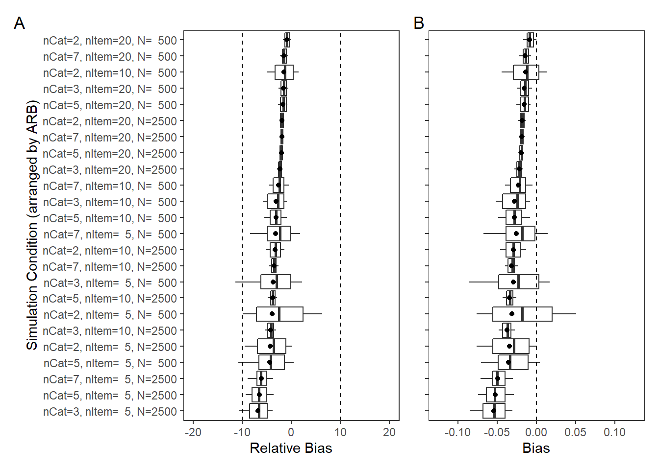
ggsave(filename = "fig/study2_parameter_bias_omega_2357.pdf",plot=p,width = 7, height=4,units="in")Warning: Removed 5 rows containing non-finite values (stat_summary).
Warning: Removed 11 rows containing non-finite values (stat_summary).ggsave(filename = "fig/study2_parameter_bias_omega_2357.png",plot=p,width = 7, height=4,units="in")Warning: Removed 5 rows containing non-finite values (stat_summary).
Warning: Removed 11 rows containing non-finite values (stat_summary).ggsave(filename = "fig/study2_parameter_bias_omega_2357.eps",plot=p,width = 7, height=4,units="in")Warning: Removed 5 rows containing non-finite values (stat_summary).
Warning: Removed 11 rows containing non-finite values (stat_summary).# visualize bias estimates
rb <- mydata %>%
filter(parameter_group == "omega", N_cat%in%c(2,5)) %>%
group_by(condition, N_cat, N_items, N) %>%
mutate(Post_Median_ARB = mean(post_median_rb_est),
Post_Median_AB = mean(post_median_bias_est))
# Create summary stats for plotting
rb_tbl <- rb %>%
group_by(condition, condition_lbs, N_cat, N_items, N) %>%
summarise(Post_Median_ARB = mean(post_median_rb_est),
Post_Median_AB = mean(post_median_bias_est)) %>%
arrange(Post_Median_ARB)`summarise()` has grouped output by 'condition', 'condition_lbs', 'N_cat', 'N_items'. You can override using the `.groups` argument.rb_tbl$lbs = factor(
rb_tbl$condition_lbs,
levels=rb_tbl$condition_lbs,
ordered=T
)
rb$lbs <- factor(
rb$condition_lbs,
levels=rb_tbl$condition_lbs,
ordered=T
)
p1 <- ggplot() +
stat_summary(
data = rb,
aes(y = lbs, x = post_median_rb_est,
group = lbs),
fun.data = cust.boxplot,
geom = "boxplot"
) +
geom_point(data = rb_tbl,
aes(y = lbs, x = Post_Median_ARB),
color = "black") +
geom_vline(xintercept = -10,
linetype = "dashed") +
geom_vline(xintercept = 10,
linetype = "dashed") +
lims(x = c(-20, 20)) +
labs(y="Simulation Condition (arranged by ARB)",
x="Relative Bias")+
theme_bw() +
theme(panel.grid = element_blank())
p2 <- ggplot() +
stat_summary(
data = rb,
aes(y = lbs, x = post_median_bias_est,
group = lbs),
fun.data = cust.boxplot,
geom = "boxplot"
) +
geom_point(data = rb_tbl,
aes(y = lbs, x = Post_Median_AB),
color = "black") +
geom_vline(xintercept = 0,
linetype = "dashed")+
lims(x = c(-0.125, 0.125)) +
labs(x="Bias")+
theme_bw() +
theme(panel.grid = element_blank(),
axis.text.y = element_blank(),
axis.title.y = element_blank())
p <- p1 + p2 + plot_layout(guides="collect") + plot_annotation(tag_levels = "A")
pWarning: Removed 4 rows containing non-finite values (stat_summary).Warning: Removed 8 rows containing non-finite values (stat_summary).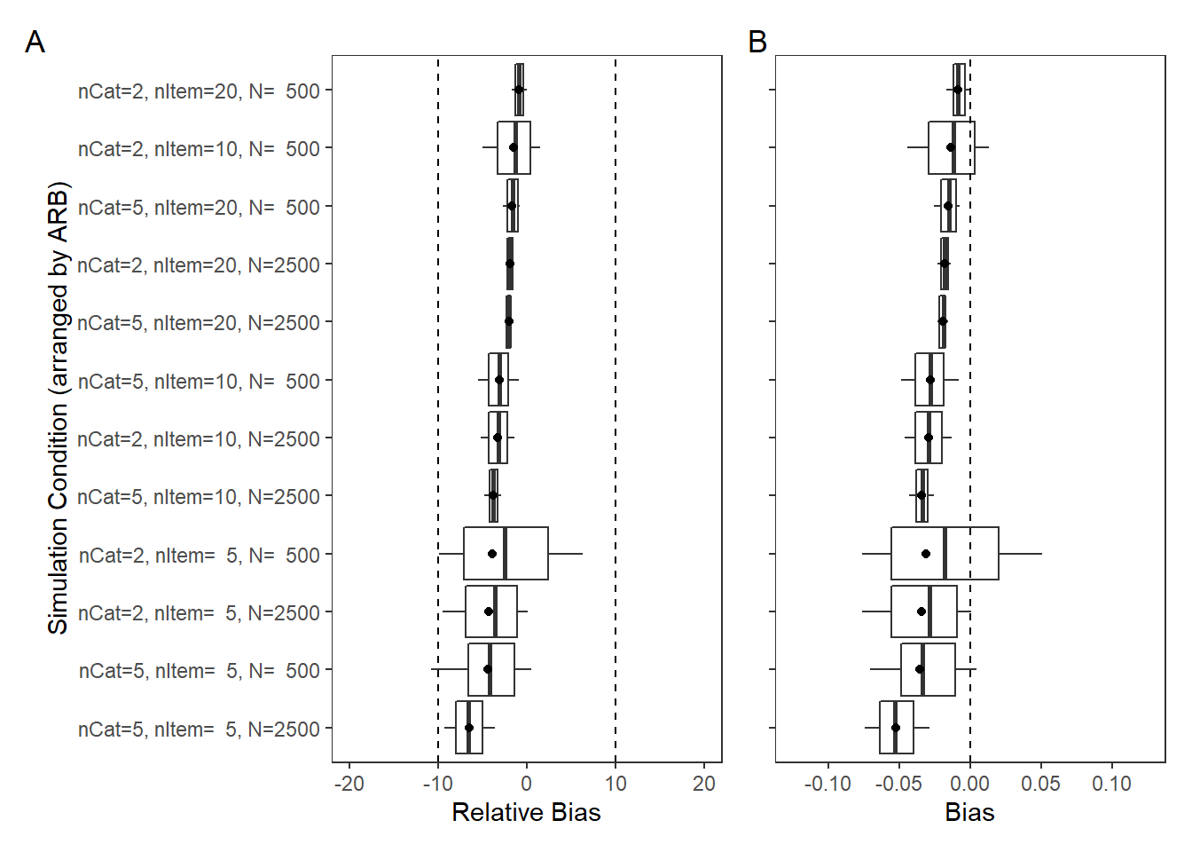
ggsave(filename = "fig/study2_parameter_bias_omega_25.pdf",plot=p,width = 7, height=4,units="in")Warning: Removed 4 rows containing non-finite values (stat_summary).
Warning: Removed 8 rows containing non-finite values (stat_summary).ggsave(filename = "fig/study2_parameter_bias_omega_25.png",plot=p,width = 7, height=4,units="in")Warning: Removed 4 rows containing non-finite values (stat_summary).
Warning: Removed 8 rows containing non-finite values (stat_summary).ggsave(filename = "fig/study2_parameter_bias_omega_25.eps",plot=p,width = 7, height=4,units="in")Warning: Removed 4 rows containing non-finite values (stat_summary).
Warning: Removed 8 rows containing non-finite values (stat_summary).
sessionInfo()R version 4.0.5 (2021-03-31)
Platform: x86_64-w64-mingw32/x64 (64-bit)
Running under: Windows 10 x64 (build 22000)
Matrix products: default
locale:
[1] LC_COLLATE=English_United States.1252
[2] LC_CTYPE=English_United States.1252
[3] LC_MONETARY=English_United States.1252
[4] LC_NUMERIC=C
[5] LC_TIME=English_United States.1252
attached base packages:
[1] stats graphics grDevices utils datasets methods base
other attached packages:
[1] car_3.0-10 carData_3.0-4 mvtnorm_1.1-1
[4] LaplacesDemon_16.1.4 runjags_2.2.0-2 lme4_1.1-26
[7] Matrix_1.3-2 sirt_3.9-4 R2jags_0.6-1
[10] rjags_4-12 eRm_1.0-2 diffIRT_1.5
[13] statmod_1.4.35 xtable_1.8-4 kableExtra_1.3.4
[16] lavaan_0.6-7 polycor_0.7-10 bayesplot_1.8.0
[19] ggmcmc_1.5.1.1 coda_0.19-4 data.table_1.14.0
[22] patchwork_1.1.1 forcats_0.5.1 stringr_1.4.0
[25] dplyr_1.0.5 purrr_0.3.4 readr_1.4.0
[28] tidyr_1.1.3 tibble_3.1.0 ggplot2_3.3.5
[31] tidyverse_1.3.0 workflowr_1.6.2
loaded via a namespace (and not attached):
[1] minqa_1.2.4 TAM_3.5-19 colorspace_2.0-0 rio_0.5.26
[5] ellipsis_0.3.1 ggridges_0.5.3 rprojroot_2.0.2 fs_1.5.0
[9] rstudioapi_0.13 farver_2.1.0 fansi_0.4.2 lubridate_1.7.10
[13] xml2_1.3.2 splines_4.0.5 mnormt_2.0.2 knitr_1.31
[17] jsonlite_1.7.2 nloptr_1.2.2.2 broom_0.7.5 dbplyr_2.1.0
[21] compiler_4.0.5 httr_1.4.2 backports_1.2.1 assertthat_0.2.1
[25] cli_2.3.1 later_1.1.0.1 htmltools_0.5.1.1 tools_4.0.5
[29] gtable_0.3.0 glue_1.4.2 Rcpp_1.0.7 cellranger_1.1.0
[33] jquerylib_0.1.3 vctrs_0.3.6 svglite_2.0.0 nlme_3.1-152
[37] psych_2.0.12 xfun_0.21 ps_1.6.0 openxlsx_4.2.3
[41] rvest_1.0.0 lifecycle_1.0.0 MASS_7.3-53.1 scales_1.1.1
[45] ragg_1.1.1 hms_1.0.0 promises_1.2.0.1 parallel_4.0.5
[49] RColorBrewer_1.1-2 curl_4.3 yaml_2.2.1 sass_0.3.1
[53] reshape_0.8.8 stringi_1.5.3 highr_0.8 zip_2.1.1
[57] boot_1.3-27 rlang_0.4.10 pkgconfig_2.0.3 systemfonts_1.0.1
[61] evaluate_0.14 lattice_0.20-41 labeling_0.4.2 tidyselect_1.1.0
[65] GGally_2.1.1 plyr_1.8.6 magrittr_2.0.1 R6_2.5.0
[69] generics_0.1.0 DBI_1.1.1 foreign_0.8-81 pillar_1.5.1
[73] haven_2.3.1 withr_2.4.1 abind_1.4-5 modelr_0.1.8
[77] crayon_1.4.1 utf8_1.1.4 tmvnsim_1.0-2 rmarkdown_2.7
[81] grid_4.0.5 readxl_1.3.1 CDM_7.5-15 pbivnorm_0.6.0
[85] git2r_0.28.0 reprex_1.0.0 digest_0.6.27 webshot_0.5.2
[89] httpuv_1.5.5 textshaping_0.3.1 stats4_4.0.5 munsell_0.5.0
[93] viridisLite_0.3.0 bslib_0.2.4 R2WinBUGS_2.1-21