Study 4: Extroversion Data Analysis
Model 3 Results
R. Noah Padgett
2022-01-17
Last updated: 2022-01-20
Checks: 4 2
Knit directory: Padgett-Dissertation/
This reproducible R Markdown analysis was created with workflowr (version 1.6.2). The Checks tab describes the reproducibility checks that were applied when the results were created. The Past versions tab lists the development history.
Great job! The global environment was empty. Objects defined in the global environment can affect the analysis in your R Markdown file in unknown ways. For reproduciblity it’s best to always run the code in an empty environment.
The command set.seed(20210401) was run prior to running the code in the R Markdown file. Setting a seed ensures that any results that rely on randomness, e.g. subsampling or permutations, are reproducible.
Great job! Recording the operating system, R version, and package versions is critical for reproducibility.
- model3
- study4-model3-ppd
To ensure reproducibility of the results, delete the cache directory study4_model3_results_cache and re-run the analysis. To have workflowr automatically delete the cache directory prior to building the file, set delete_cache = TRUE when running wflow_build() or wflow_publish().
Great job! Using relative paths to the files within your workflowr project makes it easier to run your code on other machines.
Tracking code development and connecting the code version to the results is critical for reproducibility. To start using Git, open the Terminal and type git init in your project directory.
This project is not being versioned with Git. To obtain the full reproducibility benefits of using workflowr, please see ?wflow_start.
# Load packages & utility functions
source("code/load_packages.R")
source("code/load_utility_functions.R")
# environment options
options(scipen = 999, digits=3)
Describing the Observed Data
# Load diffIRT package with data
library(diffIRT)
data("extraversion")
mydata <- na.omit(extraversion)

# separate data then recombine
d1 <- mydata %>%
  as.data.frame() %>%
  select(contains("X"))%>%
  mutate(id = 1:n()) %>%
  pivot_longer(
    cols=contains("X"),
    names_to = c("item"),
    values_to = "Response"
  ) %>%
  mutate(
    item = ifelse(nchar(item)==4,substr(item, 3,3),substr(item, 3,4))
  )
d2 <- mydata %>%
  as.data.frame() %>%
  select(contains("T"))%>%
  mutate(id = 1:n()) %>%
  pivot_longer(
    cols=starts_with("T"),
    names_to = c("item"),
    values_to = "Time"
  ) %>%
  mutate(
    item = ifelse(nchar(item)==4,substr(item, 3,3),substr(item, 3,4))
  )
dat <- left_join(d1, d2)
Joining, by = c("id", "item")dat_sum <- dat %>%
select(item, Response, Time) %>%
group_by(item) %>%
summarize(
M1 = mean(Response, na.rm=T),
Mt = mean(Time, na.rm=T),
SDt = sd(Time, na.rm=T),
Mlogt = mean(log(Time), na.rm=T),
)
colnames(dat_sum) <-
c(
"Item",
"Proportion Endorsed",
"Mean Response Time",
"SD Response Time",
"Mean Log Response Time"
)
kable(dat_sum, format = "html", digits = 3) %>%
kable_styling(full_width = T)| Item | Proportion Endorsed | Mean Response Time | SD Response Time | Mean Log Response Time |
|---|---|---|---|---|
| 1 | 0.739 | 1.488 | 0.805 | 0.288 |
| 10 | 0.866 | 0.979 | 0.520 | -0.115 |
| 2 | 0.535 | 1.354 | 0.648 | 0.208 |
| 3 | 0.852 | 1.115 | 0.632 | 0.002 |
| 4 | 0.923 | 1.001 | 0.664 | -0.114 |
| 5 | 0.542 | 1.301 | 0.706 | 0.163 |
| 6 | 0.901 | 1.255 | 0.682 | 0.119 |
| 7 | 0.944 | 1.143 | 0.546 | 0.054 |
| 8 | 0.965 | 1.067 | 0.575 | -0.030 |
| 9 | 0.824 | 1.728 | 0.745 | 0.463 |
# covariance among items
kable(cov(mydata[,colnames(mydata) %like% "X"]), digits = 3) %>%
kable_styling(full_width = T)| X[1] | X[2] | X[3] | X[4] | X[5] | X[6] | X[7] | X[8] | X[9] | X[10] | |
|---|---|---|---|---|---|---|---|---|---|---|
| X[1] | 0.194 | -0.001 | 0.039 | 0.029 | 0.000 | 0.002 | 0.014 | 0.005 | 0.011 | 0.015 |
| X[2] | -0.001 | 0.251 | 0.023 | 0.006 | 0.077 | 0.011 | 0.002 | 0.012 | 0.031 | 0.030 |
| X[3] | 0.039 | 0.023 | 0.127 | 0.038 | 0.024 | 0.028 | 0.020 | 0.016 | 0.016 | 0.051 |
| X[4] | 0.029 | 0.006 | 0.038 | 0.072 | 0.014 | 0.006 | 0.017 | 0.019 | 0.029 | 0.025 |
| X[5] | 0.000 | 0.077 | 0.024 | 0.014 | 0.250 | 0.004 | 0.017 | 0.005 | 0.032 | 0.031 |
| X[6] | 0.002 | 0.011 | 0.028 | 0.006 | 0.004 | 0.090 | 0.009 | 0.011 | 0.004 | 0.015 |
| X[7] | 0.014 | 0.002 | 0.020 | 0.017 | 0.017 | 0.009 | 0.054 | 0.019 | 0.004 | 0.007 |
| X[8] | 0.005 | 0.012 | 0.016 | 0.019 | 0.005 | 0.011 | 0.019 | 0.034 | 0.008 | 0.009 |
| X[9] | 0.011 | 0.031 | 0.016 | 0.029 | 0.032 | 0.004 | 0.004 | 0.008 | 0.146 | 0.033 |
| X[10] | 0.015 | 0.030 | 0.051 | 0.025 | 0.031 | 0.015 | 0.007 | 0.009 | 0.033 | 0.117 |
# correlation matrix
psych::polychoric(mydata[,colnames(mydata) %like% "X"])
Warning in cor.smooth(mat): Matrix was not positive definite, smoothing was doneCall: psych::polychoric(x = mydata[, colnames(mydata) %like% "X"])
Polychoric correlations
X[1] X[2] X[3] X[4] X[5] X[6] X[7] X[8] X[9] X[10]
X[1] 1.00
X[2] -0.01 1.00
X[3] 0.45 0.24 1.00
X[4] 0.50 0.11 0.70 1.00
X[5] 0.00 0.46 0.26 0.23 1.00
X[6] 0.04 0.15 0.50 0.21 0.06 1.00
X[7] 0.32 0.05 0.52 0.58 0.36 0.32 1.00
X[8] 0.18 0.38 0.57 0.71 0.17 0.48 0.78 1.00
X[9] 0.12 0.29 0.24 0.55 0.31 0.08 0.13 0.31 1.00
X[10] 0.19 0.34 0.69 0.54 0.35 0.32 0.22 0.39 0.47 1.00
with tau of
1
X[1] -0.642
X[2] -0.088
X[3] -1.046
X[4] -1.422
X[5] -0.106
X[6] -1.290
X[7] -1.586
X[8] -1.809
X[9] -0.930
X[10] -1.109Model 3: IFA with RT only
Model details
cat(read_file(paste0(w.d, "/code/study_4/model_3.txt")))model {
### Model
for(p in 1:N){
for(i in 1:nit){
# data model
y[p,i] ~ dbern(omega[p,i,2])
# LRV
ystar[p,i] ~ dnorm(lambda[i]*eta[p], 1)
# Pr(nu = 2)
pi[p,i,2] = phi(ystar[p,i] - tau[i,1])
# Pr(nu = 1)
pi[p,i,1] = 1 - phi(ystar[p,i] - tau[i,1])
# MISCLASSIFICATION MODEL
for(c in 1:ncat){
# generate informative prior for misclassificaiton
# parameters based on RT
for(ct in 1:ncat){
alpha[p,i,ct,c] <- ifelse(c == ct,
ilogit(lrt[p,i]),
(1/(ncat-1))*(1-ilogit(lrt[p,i]))
)
}
# sample misclassification parameters using the informative priors
gamma[p,i,c,1:ncat] ~ ddirch(alpha[p,i,c,1:ncat])
# observed category prob (Pr(y=c))
omega[p,i, c] = gamma[p,i,c,1]*pi[p,i,1] +
gamma[p,i,c,2]*pi[p,i,2]
}
}
}
### Priors
# person parameters
for(p in 1:N){
eta[p] ~ dnorm(0, 1) # latent ability
}
for(i in 1:nit){
# Thresholds
tau[i, 1] ~ dnorm(0.0,0.1)
# loadings
lambda[i] ~ dnorm(0, .44)T(0,)
# LRV total variance
# total variance = residual variance + fact. Var.
theta[i] = 1 + pow(lambda[i],2)
# standardized loading
lambda.std[i] = lambda[i]/pow(theta[i],0.5)
}
# compute omega
lambda_sum[1] = lambda[1]
for(i in 2:nit){
#lambda_sum (sum factor loadings)
lambda_sum[i] = lambda_sum[i-1]+lambda[i]
}
reli.omega = (pow(lambda_sum[nit],2))/(pow(lambda_sum[nit],2)+nit)
}Model results
# Save parameters
jags.params <- c("tau", "lambda", "theta", "reli.omega", "lambda.std")
# initial-values
jags.inits <- function(){
    list(
      "tau"=matrix(c(-0.64, -0.09, -1.05, -1.42, -0.11, -1.29, -1.59, -1.81, -0.93, -1.11),
                   ncol=1, nrow=10),
      "lambda"=rep(0.7,10),
      "eta"=rnorm(142),
      "ystar"=matrix(c(0.7*rep(rnorm(142),10)), ncol=10)
    )
  }
jags.data <- list(
  y = mydata[,1:10],
  lrt = mydata[,11:20],
  N = nrow(mydata),
  nit = 10,
  ncat = 2
)
model.fit <-  R2jags::jags(
  model = paste0(w.d, "/code/study_4/model_3.txt"),
  parameters.to.save = jags.params,
  data = jags.data,
  n.chains = 4,
  n.burnin = 5000,
  n.iter = 10000
)
module glm loadedCompiling model graph
Resolving undeclared variables
Allocating nodes
Graph information:
Observed stochastic nodes: 1420
Unobserved stochastic nodes: 4422
Total graph size: 34704
Initializing modelprint(model.fit, width=1000)Inference for Bugs model at "C:/Users/noahp/Documents/GitHub/Padgett-Dissertation/code/study_4/model_3.txt", fit using jags,
4 chains, each with 10000 iterations (first 5000 discarded), n.thin = 5
n.sims = 4000 iterations saved
mu.vect sd.vect 2.5% 25% 50% 75% 97.5% Rhat n.eff
lambda[1] 1.650 0.910 0.248 0.986 1.514 2.192 3.845 1.03 290
lambda[2] 2.023 0.886 0.616 1.334 1.946 2.614 3.895 1.06 51
lambda[3] 1.984 0.750 0.559 1.462 1.955 2.493 3.446 1.04 260
lambda[4] 1.608 0.957 0.078 0.852 1.560 2.233 3.653 1.13 28
lambda[5] 1.413 0.701 0.333 0.905 1.310 1.814 3.122 1.05 66
lambda[6] 0.728 0.555 0.026 0.289 0.611 1.032 2.083 1.00 770
lambda[7] 0.829 0.629 0.034 0.332 0.714 1.179 2.307 1.02 130
lambda[8] 0.812 0.635 0.034 0.322 0.667 1.161 2.415 1.03 100
lambda[9] 1.481 0.764 0.224 0.930 1.415 1.930 3.266 1.10 42
lambda[10] 1.792 0.822 0.263 1.214 1.768 2.358 3.528 1.09 47
lambda.std[1] 0.774 0.188 0.241 0.702 0.834 0.910 0.968 1.06 160
lambda.std[2] 0.848 0.121 0.525 0.800 0.889 0.934 0.969 1.06 74
lambda.std[3] 0.853 0.122 0.488 0.825 0.890 0.928 0.960 1.08 200
lambda.std[4] 0.742 0.239 0.078 0.649 0.842 0.913 0.965 1.11 45
lambda.std[5] 0.752 0.166 0.316 0.671 0.795 0.876 0.952 1.06 94
lambda.std[6] 0.497 0.261 0.026 0.278 0.521 0.718 0.901 1.00 1500
lambda.std[7] 0.534 0.267 0.034 0.315 0.581 0.763 0.918 1.02 160
lambda.std[8] 0.525 0.266 0.034 0.307 0.555 0.758 0.924 1.03 130
lambda.std[9] 0.755 0.187 0.218 0.681 0.817 0.888 0.956 1.14 52
lambda.std[10] 0.810 0.173 0.254 0.772 0.870 0.921 0.962 1.13 65
reli.omega 0.950 0.016 0.911 0.941 0.953 0.962 0.974 1.19 18
tau[1,1] -1.951 0.870 -4.334 -2.317 -1.747 -1.365 -0.868 1.08 66
tau[2,1] 0.026 0.436 -0.863 -0.244 0.024 0.297 0.904 1.02 200
tau[3,1] -3.211 0.895 -5.196 -3.761 -3.114 -2.572 -1.774 1.01 590
tau[4,1] -3.983 1.287 -7.167 -4.710 -3.742 -3.036 -2.153 1.14 27
tau[5,1] -0.260 0.407 -1.122 -0.503 -0.242 0.000 0.499 1.05 60
tau[6,1] -4.846 1.665 -8.785 -5.794 -4.568 -3.580 -2.479 1.02 120
tau[7,1] -4.855 1.492 -8.325 -5.677 -4.592 -3.758 -2.702 1.02 140
tau[8,1] -5.305 1.611 -9.217 -6.168 -5.015 -4.147 -2.984 1.01 250
tau[9,1] -2.898 0.937 -5.136 -3.434 -2.741 -2.223 -1.508 1.04 69
tau[10,1] -3.448 1.053 -5.890 -4.027 -3.297 -2.677 -1.859 1.02 150
theta[1] 4.551 3.765 1.062 1.973 3.292 5.804 15.781 1.02 670
theta[2] 5.876 4.074 1.380 2.779 4.786 7.833 16.170 1.06 49
theta[3] 5.498 3.151 1.313 3.137 4.823 7.216 12.878 1.01 460
theta[4] 4.500 3.713 1.006 1.726 3.433 5.988 14.347 1.17 21
theta[5] 3.488 2.450 1.111 1.819 2.715 4.289 10.749 1.05 59
theta[6] 1.838 1.189 1.001 1.084 1.373 2.066 5.337 1.03 160
theta[7] 2.083 1.562 1.001 1.111 1.510 2.391 6.322 1.03 110
theta[8] 2.063 1.656 1.001 1.104 1.445 2.349 6.830 1.03 91
theta[9] 3.777 2.820 1.050 1.865 3.003 4.725 11.664 1.06 46
theta[10] 4.888 3.281 1.069 2.474 4.127 6.560 13.448 1.06 47
deviance 906.111 40.987 827.567 878.036 905.952 934.364 985.376 1.04 71
For each parameter, n.eff is a crude measure of effective sample size,
and Rhat is the potential scale reduction factor (at convergence, Rhat=1).
DIC info (using the rule, pD = var(deviance)/2)
pD = 804.9 and DIC = 1711.1
DIC is an estimate of expected predictive error (lower deviance is better).Posterior Distribution Summary
jags.mcmc <- as.mcmc(model.fit)
a <- colnames(as.data.frame(jags.mcmc[[1]]))
fit.mcmc <- data.frame(as.matrix(jags.mcmc, chains = T, iters = T))
colnames(fit.mcmc) <- c("chain", "iter", a)
fit.mcmc.ggs <- ggmcmc::ggs(jags.mcmc) # for GRB plot

# save posterior draws for later
write.csv(x=fit.mcmc, file=paste0(getwd(),"/data/study_4/posterior_draws_m3.csv"))
Categroy Thresholds (\(\tau\))
# tau
bayesplot::mcmc_areas(fit.mcmc, regex_pars = "tau", prob = 0.8); ggsave("fig/study4_model3_tau_dens.pdf")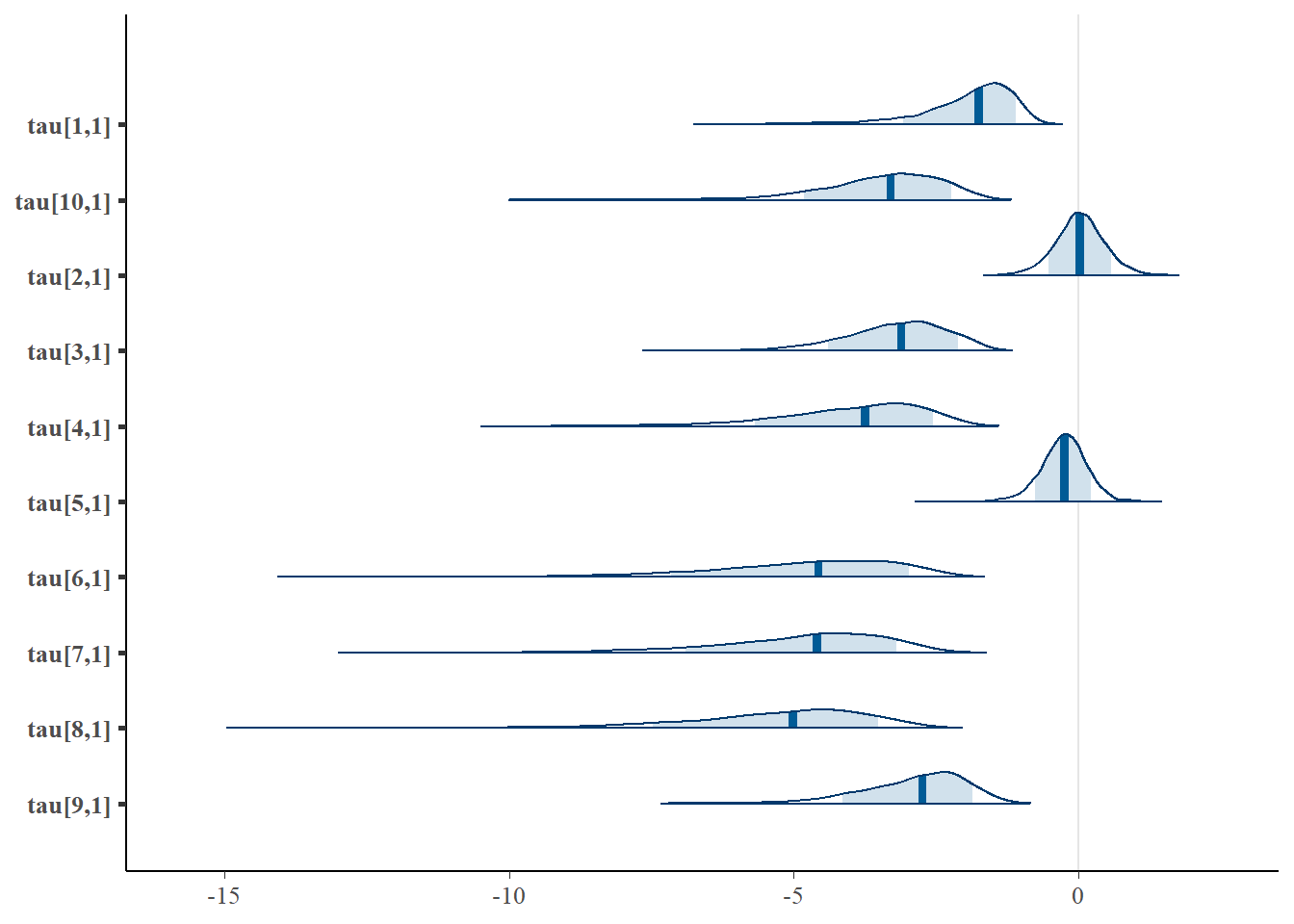
Saving 7 x 5 in imagebayesplot::mcmc_acf(fit.mcmc, regex_pars = "tau"); ggsave("fig/study4_model3_tau_acf.pdf")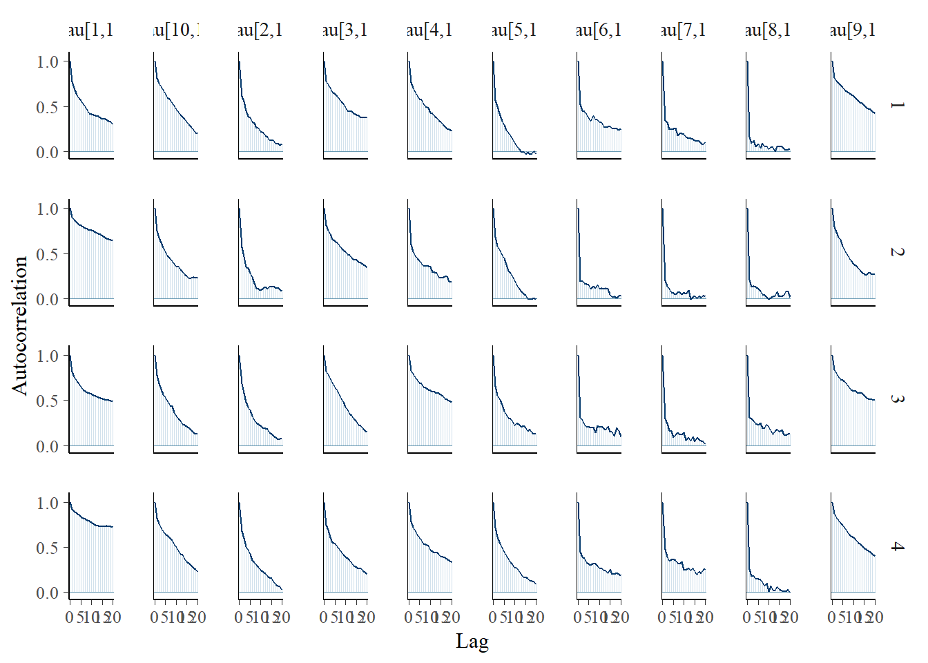
Saving 7 x 5 in imagebayesplot::mcmc_trace(fit.mcmc, regex_pars = "tau"); ggsave("fig/study4_model3_tau_trace.pdf")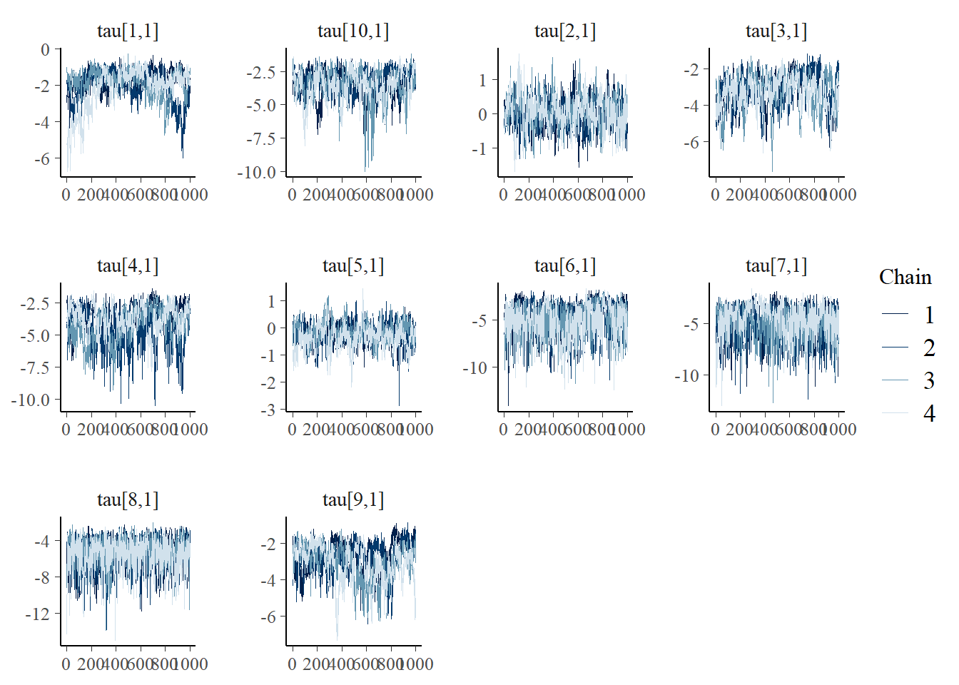
Saving 7 x 5 in imageggmcmc::ggs_grb(fit.mcmc.ggs, family = "tau"); ggsave("fig/study4_model3_tau_grb.pdf")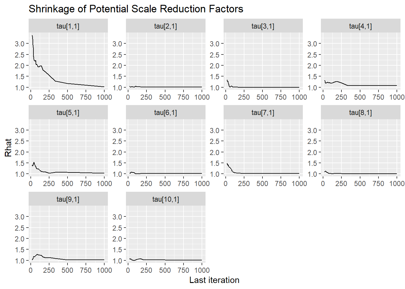
Saving 7 x 5 in imageFactor Loadings (\(\lambda\))
bayesplot::mcmc_areas(fit.mcmc, regex_pars = "lambda", prob = 0.8)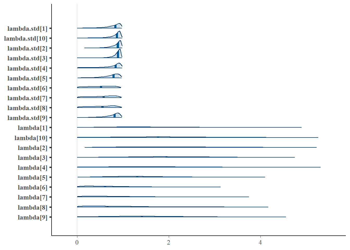
bayesplot::mcmc_acf(fit.mcmc, regex_pars = "lambda")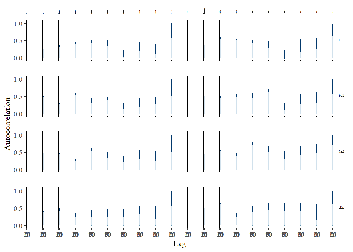
bayesplot::mcmc_trace(fit.mcmc, regex_pars = "lambda")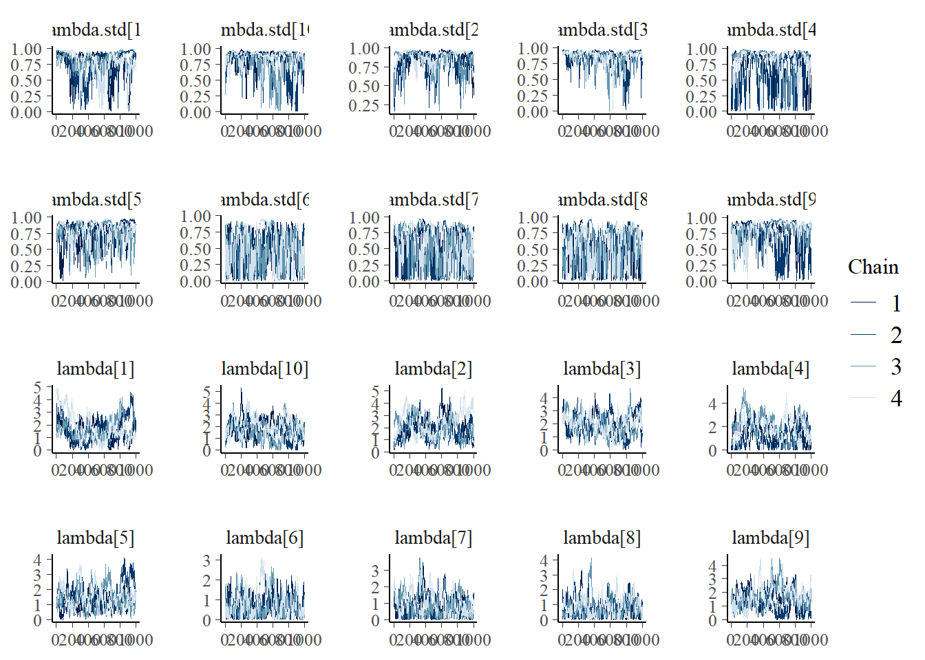
ggmcmc::ggs_grb(fit.mcmc.ggs, family = "lambda")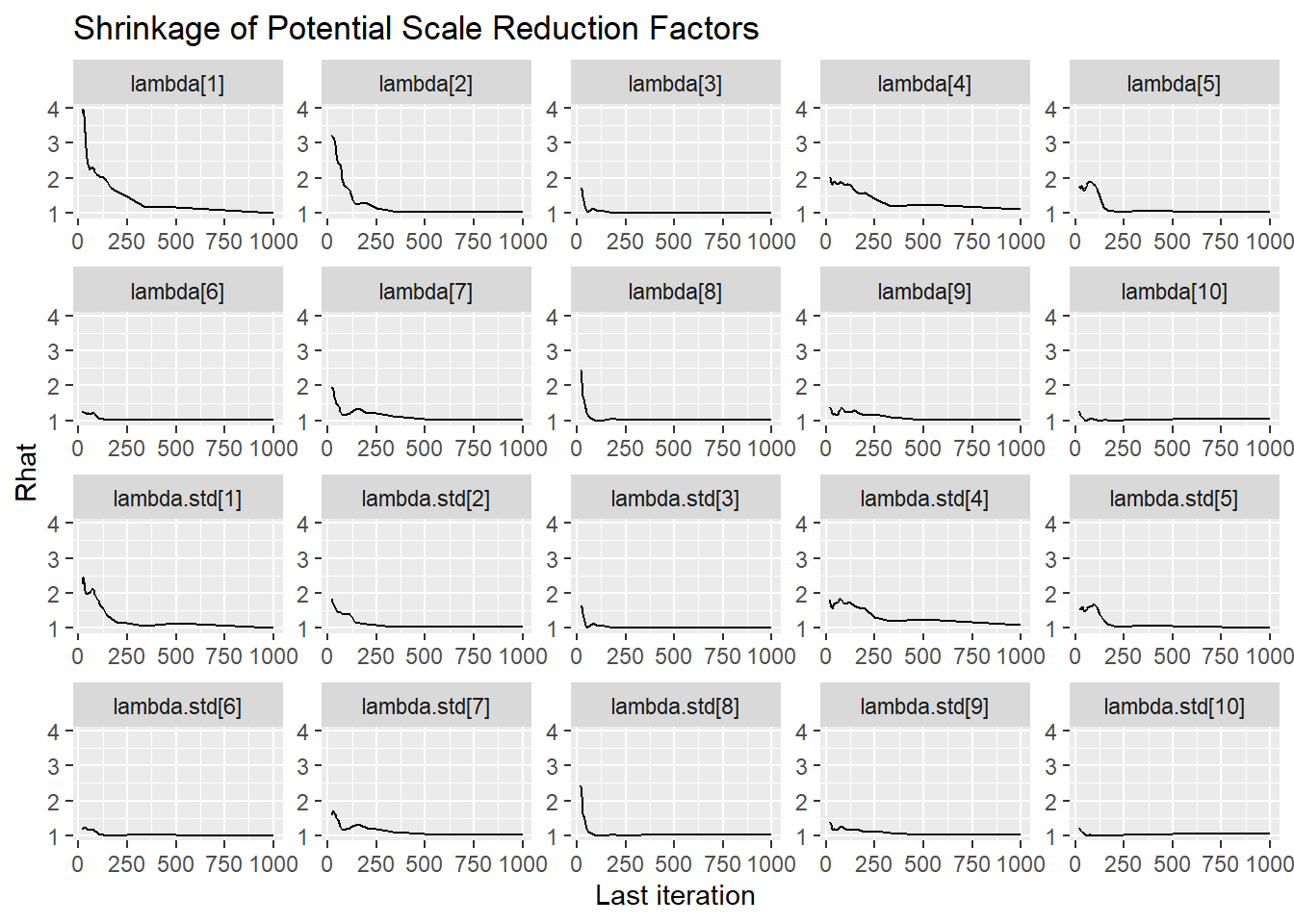
bayesplot::mcmc_areas(fit.mcmc, regex_pars = "lambda.std", prob = 0.8); ggsave("fig/study4_model3_lambda_dens.pdf")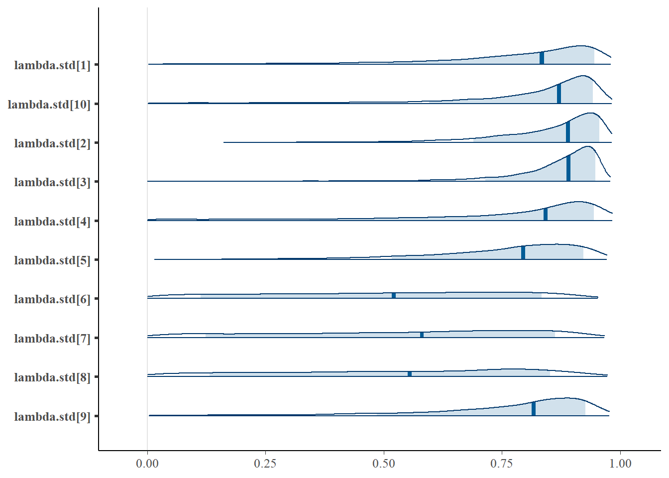
Saving 7 x 5 in imagebayesplot::mcmc_acf(fit.mcmc, regex_pars = "lambda.std"); ggsave("fig/study4_model3_lambda_acf.pdf")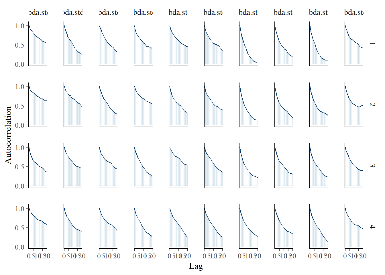
Saving 7 x 5 in imagebayesplot::mcmc_trace(fit.mcmc, regex_pars = "lambda.std"); ggsave("fig/study4_model3_lambda_trace.pdf")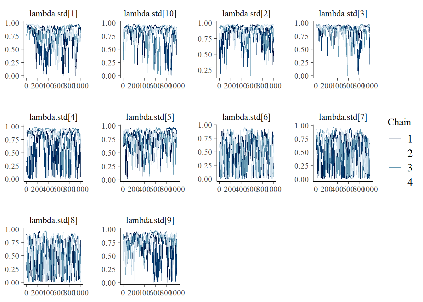
Saving 7 x 5 in imageggmcmc::ggs_grb(fit.mcmc.ggs, family = "lambda.std"); ggsave("fig/study4_model3_lambda_grb.pdf")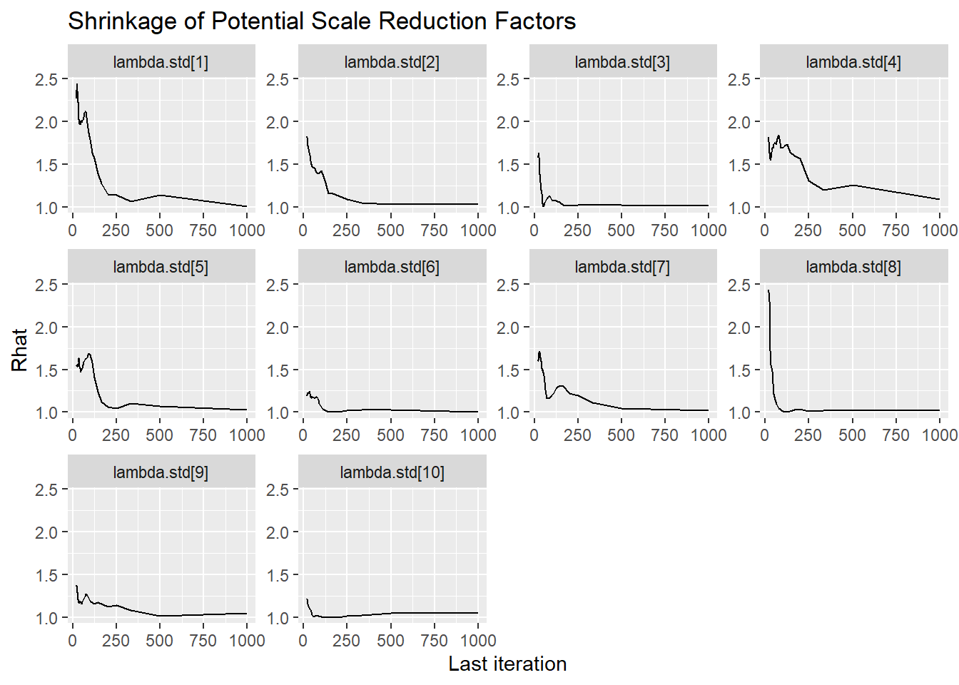
Saving 7 x 5 in imageLatent Response Total Variance (\(\theta\))
bayesplot::mcmc_areas(fit.mcmc, regex_pars = "theta", prob = 0.8); ggsave("fig/study4_model3_theta_dens.pdf")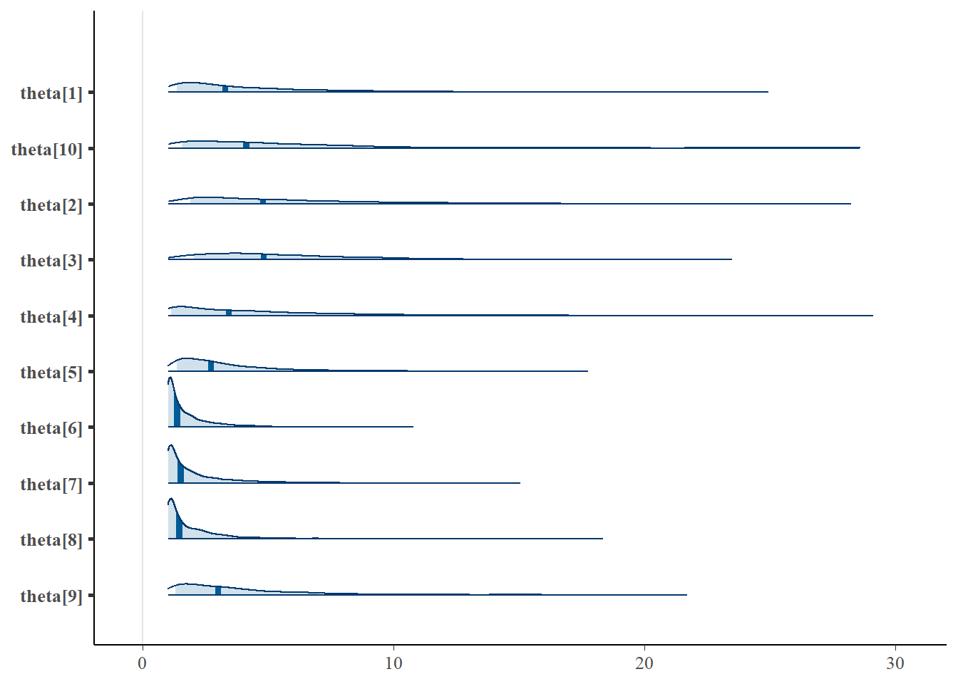
Saving 7 x 5 in imagebayesplot::mcmc_acf(fit.mcmc, regex_pars = "theta"); ggsave("fig/study4_model3_theta_acf.pdf")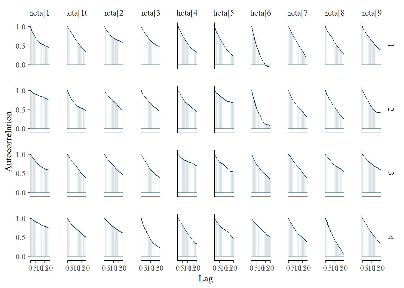
Saving 7 x 5 in imagebayesplot::mcmc_trace(fit.mcmc, regex_pars = "theta"); ggsave("fig/study4_model3_theta_trace.pdf")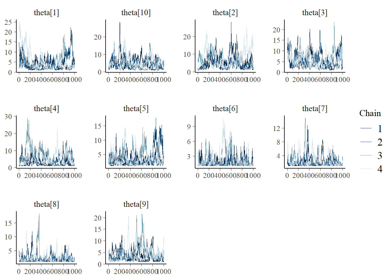
Saving 7 x 5 in imageggmcmc::ggs_grb(fit.mcmc.ggs, family = "theta"); ggsave("fig/study4_model3_theta_grb.pdf")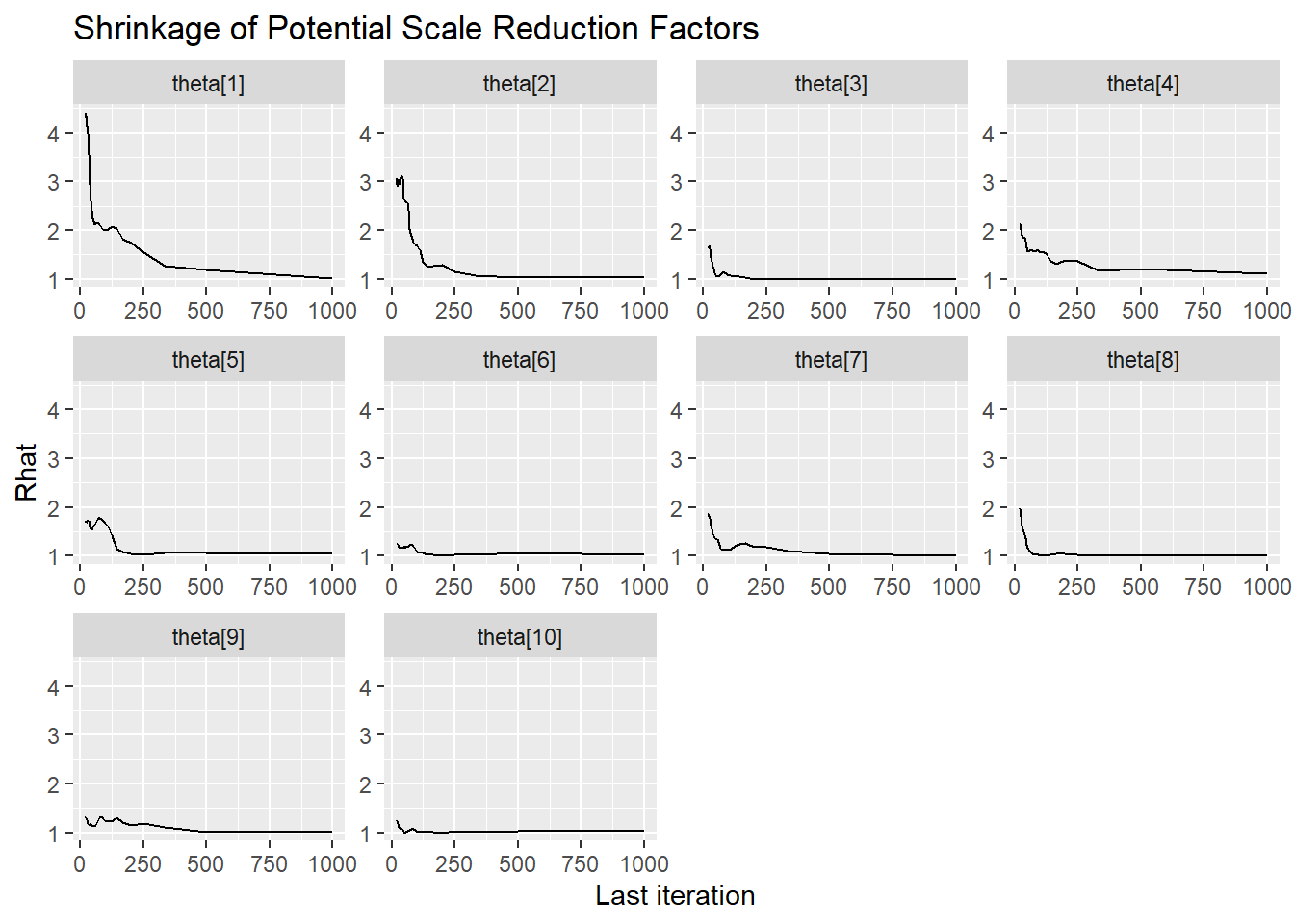
Saving 7 x 5 in imageFactor Reliability Omega (\(\omega\))
bayesplot::mcmc_areas(fit.mcmc, regex_pars = "reli.omega", prob = 0.8); ggsave("fig/study4_model3_omega_dens.pdf")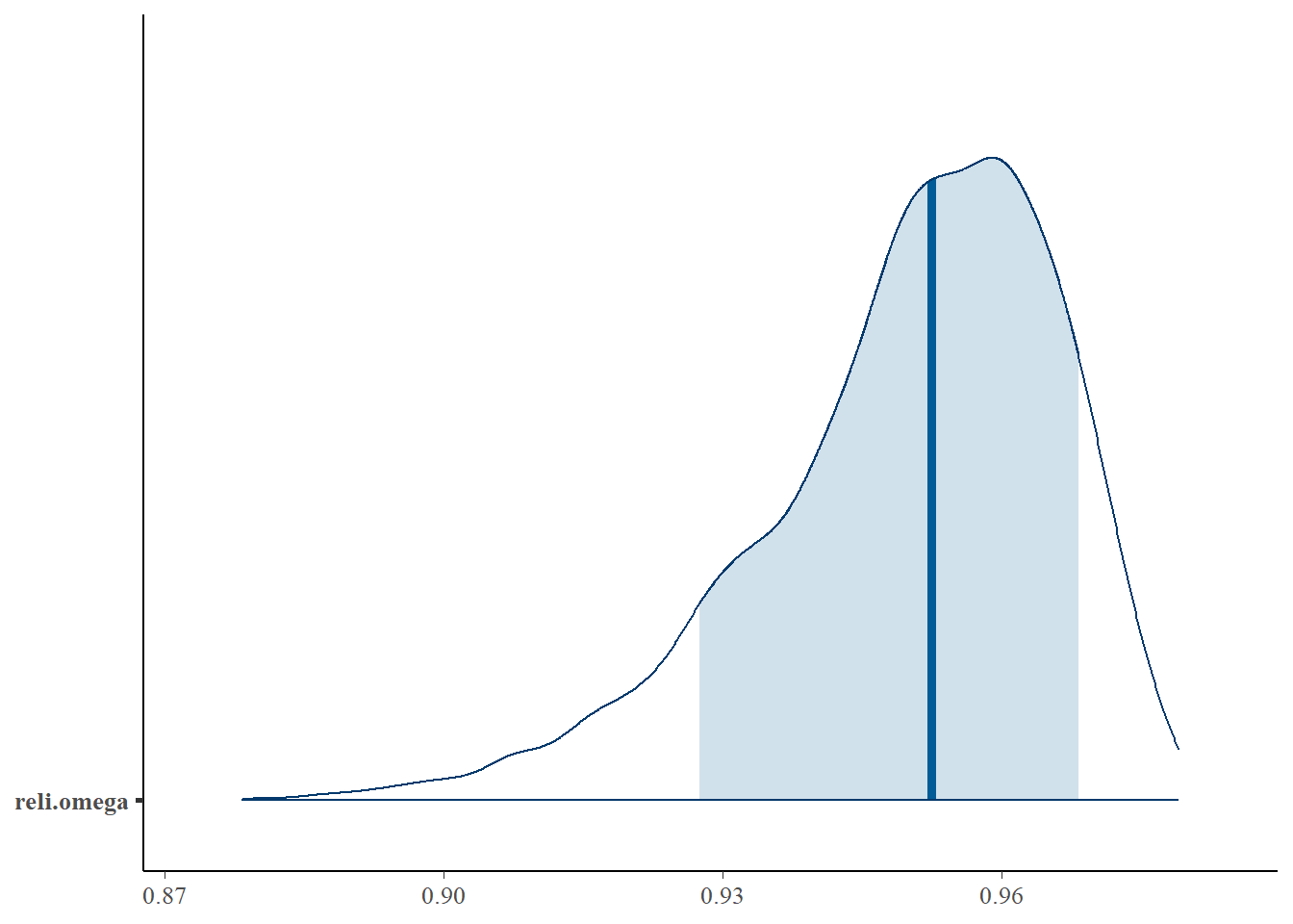
Saving 7 x 5 in imagebayesplot::mcmc_acf(fit.mcmc, regex_pars = "reli.omega"); ggsave("fig/study4_model3_omega_acf.pdf")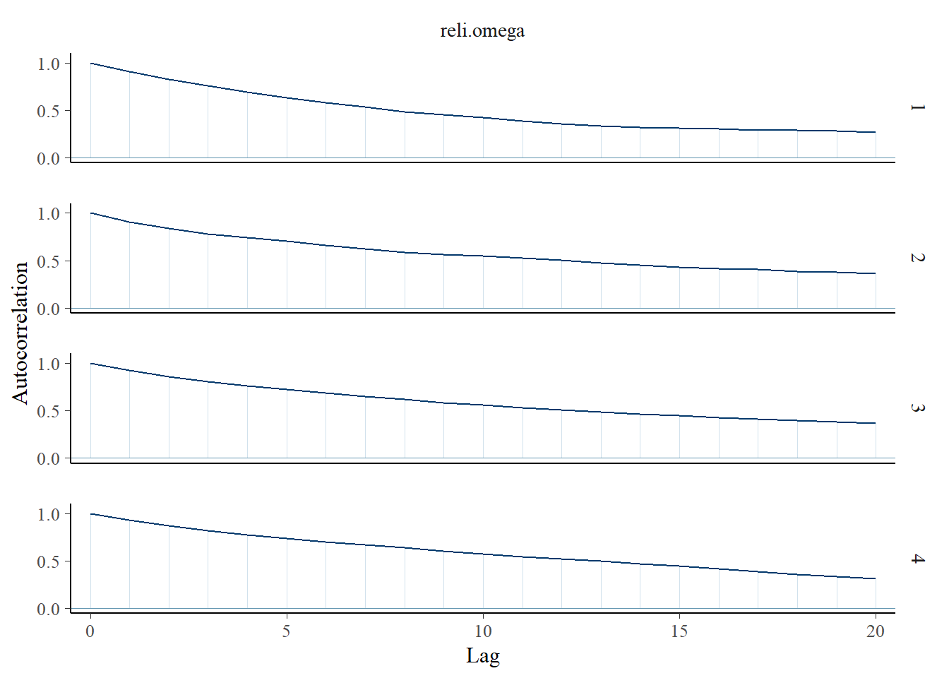
Saving 7 x 5 in imagebayesplot::mcmc_trace(fit.mcmc, regex_pars = "reli.omega"); ggsave("fig/study4_model3_omega_trace.pdf")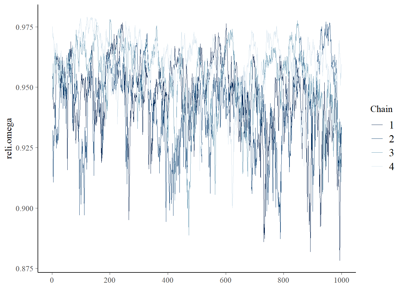
Saving 7 x 5 in imageggmcmc::ggs_grb(fit.mcmc.ggs, family = "reli.omega"); ggsave("fig/study4_model3_omega_grb.pdf")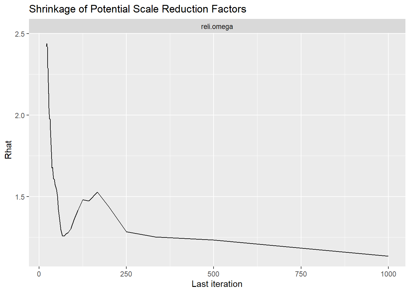
Saving 7 x 5 in image# extract omega posterior for results comparison
extracted_omega <- data.frame(model_3 = fit.mcmc$reli.omega)
write.csv(x=extracted_omega, file=paste0(getwd(),"/data/study_4/extracted_omega_m3.csv"))Posterior Predictive Distributions
# Posterior Predictive Check
Niter <- 200
model.fit$model$recompile()
Compiling model graph
Resolving undeclared variables
Allocating nodes
Graph information:
Observed stochastic nodes: 1420
Unobserved stochastic nodes: 4422
Total graph size: 34704
Initializing modelfit.extra <- rjags::jags.samples(model.fit$model, variable.names = "omega", n.iter = Niter)NOTE: Stopping adaptationN <- 142
nit <- 10
nchain<-4
C <- 2
n <- i <- iter <- ppc.row.i <- 1
y.prob.ppc <- array(dim=c(Niter*nchain, nit, C))
for(chain in 1:nchain){
for(iter in 1:Niter){
# initialize simulated y for this iteration
y <- matrix(nrow=N, ncol=nit)
# loop over item
for(i in 1:nit){
# simulated data for item i for each person
for(n in 1:N){
y[n,i] <- sample(1:C, 1, prob = fit.extra$omega[n, i, 1:C, iter, chain])
}
# computer proportion of each response category
for(c in 1:C){
y.prob.ppc[ppc.row.i,i,c] <- sum(y[,i]==c)/N
}
}
# update row of output
ppc.row.i = ppc.row.i + 1
}
}
yppcmat <- matrix(c(y.prob.ppc), ncol=1)
z <- expand.grid(1:(Niter*nchain), 1:nit, 1:C)
yppcmat <- data.frame( iter = z[,1], nit=z[,2], C=z[,3], yppc = yppcmat)
ymat <- model.fit$model$data()[["y"]]
y.prob <- matrix(ncol=C, nrow=nit)
for(i in 1:nit){
for(c in 1:C){
y.prob[i,c] <- sum(ymat[,i]==c-1)/N
}
}
yobsmat <- matrix(c(y.prob), ncol=1)
z <- expand.grid(1:nit, 1:C)
yobsmat <- data.frame(nit=z[,1], C=z[,2], yobs = yobsmat)
plot.ppc <- full_join(yppcmat, yobsmat)Joining, by = c("nit", "C")p <- plot.ppc %>%
mutate(C = as.factor(C),
item = nit) %>%
ggplot()+
geom_boxplot(aes(x=C,y=y.prob.ppc), outlier.colour = NA)+
geom_point(aes(x=C,y=yobs), color="red")+
lims(y=c(0, 1))+
labs(y="Posterior Predictive Category Proportion", x="Item Category")+
facet_wrap(.~nit, nrow=1)+
theme_bw()+
theme(
panel.grid = element_blank(),
strip.background = element_rect(fill="white")
)
p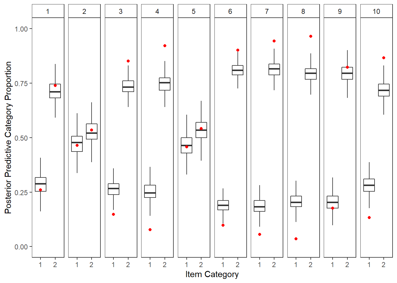
ggsave(filename = "fig/study4_model3_ppc_y.pdf",plot=p,width = 6, height=3,units="in")
ggsave(filename = "fig/study4_model3_ppc_y.png",plot=p,width = 6, height=3,units="in")
ggsave(filename = "fig/study4_model3_ppc_y.eps",plot=p,width = 6, height=3,units="in")
Manuscript Table and Figures
Table
# print to xtable
print(
  xtable(
    model.fit$BUGSoutput$summary,
    caption = c("study4 Model 3 posterior distribution summary")
    ,align = "lrrrrrrrrr"
  ),
  include.rownames=T,
  booktabs=T
)
% latex table generated in R 4.0.5 by xtable 1.8-4 package
% Thu Jan 20 14:06:05 2022
\begin{table}[ht]
\centering
\begin{tabular}{lrrrrrrrrr}
\toprule
& mean & sd & 2.5\% & 25\% & 50\% & 75\% & 97.5\% & Rhat & n.eff \\
\midrule
deviance & 906.11 & 40.99 & 827.57 & 878.04 & 905.95 & 934.36 & 985.38 & 1.04 & 71.00 \\
lambda[1] & 1.65 & 0.91 & 0.25 & 0.99 & 1.51 & 2.19 & 3.84 & 1.03 & 290.00 \\
lambda[2] & 2.02 & 0.89 & 0.62 & 1.33 & 1.95 & 2.61 & 3.89 & 1.06 & 51.00 \\
lambda[3] & 1.98 & 0.75 & 0.56 & 1.46 & 1.96 & 2.49 & 3.45 & 1.04 & 260.00 \\
lambda[4] & 1.61 & 0.96 & 0.08 & 0.85 & 1.56 & 2.23 & 3.65 & 1.13 & 28.00 \\
lambda[5] & 1.41 & 0.70 & 0.33 & 0.91 & 1.31 & 1.81 & 3.12 & 1.05 & 66.00 \\
lambda[6] & 0.73 & 0.55 & 0.03 & 0.29 & 0.61 & 1.03 & 2.08 & 1.01 & 770.00 \\
lambda[7] & 0.83 & 0.63 & 0.03 & 0.33 & 0.71 & 1.18 & 2.31 & 1.02 & 130.00 \\
lambda[8] & 0.81 & 0.64 & 0.03 & 0.32 & 0.67 & 1.16 & 2.41 & 1.03 & 100.00 \\
lambda[9] & 1.48 & 0.76 & 0.22 & 0.93 & 1.42 & 1.93 & 3.27 & 1.10 & 42.00 \\
lambda[10] & 1.79 & 0.82 & 0.26 & 1.21 & 1.77 & 2.36 & 3.53 & 1.09 & 47.00 \\
lambda.std[1] & 0.77 & 0.19 & 0.24 & 0.70 & 0.83 & 0.91 & 0.97 & 1.06 & 160.00 \\
lambda.std[2] & 0.85 & 0.12 & 0.52 & 0.80 & 0.89 & 0.93 & 0.97 & 1.06 & 74.00 \\
lambda.std[3] & 0.85 & 0.12 & 0.49 & 0.83 & 0.89 & 0.93 & 0.96 & 1.09 & 200.00 \\
lambda.std[4] & 0.74 & 0.24 & 0.08 & 0.65 & 0.84 & 0.91 & 0.96 & 1.11 & 45.00 \\
lambda.std[5] & 0.75 & 0.17 & 0.32 & 0.67 & 0.79 & 0.88 & 0.95 & 1.06 & 94.00 \\
lambda.std[6] & 0.50 & 0.26 & 0.03 & 0.28 & 0.52 & 0.72 & 0.90 & 1.00 & 1500.00 \\
lambda.std[7] & 0.53 & 0.27 & 0.03 & 0.32 & 0.58 & 0.76 & 0.92 & 1.02 & 160.00 \\
lambda.std[8] & 0.53 & 0.27 & 0.03 & 0.31 & 0.55 & 0.76 & 0.92 & 1.03 & 130.00 \\
lambda.std[9] & 0.76 & 0.19 & 0.22 & 0.68 & 0.82 & 0.89 & 0.96 & 1.14 & 52.00 \\
lambda.std[10] & 0.81 & 0.17 & 0.25 & 0.77 & 0.87 & 0.92 & 0.96 & 1.13 & 65.00 \\
reli.omega & 0.95 & 0.02 & 0.91 & 0.94 & 0.95 & 0.96 & 0.97 & 1.19 & 18.00 \\
tau[1,1] & -1.95 & 0.87 & -4.33 & -2.32 & -1.75 & -1.36 & -0.87 & 1.08 & 66.00 \\
tau[2,1] & 0.03 & 0.44 & -0.86 & -0.24 & 0.02 & 0.30 & 0.90 & 1.02 & 200.00 \\
tau[3,1] & -3.21 & 0.90 & -5.20 & -3.76 & -3.11 & -2.57 & -1.77 & 1.01 & 590.00 \\
tau[4,1] & -3.98 & 1.29 & -7.17 & -4.71 & -3.74 & -3.04 & -2.15 & 1.14 & 27.00 \\
tau[5,1] & -0.26 & 0.41 & -1.12 & -0.50 & -0.24 & 0.00 & 0.50 & 1.05 & 60.00 \\
tau[6,1] & -4.85 & 1.67 & -8.79 & -5.79 & -4.57 & -3.58 & -2.48 & 1.02 & 120.00 \\
tau[7,1] & -4.85 & 1.49 & -8.32 & -5.68 & -4.59 & -3.76 & -2.70 & 1.02 & 140.00 \\
tau[8,1] & -5.30 & 1.61 & -9.22 & -6.17 & -5.01 & -4.15 & -2.98 & 1.01 & 250.00 \\
tau[9,1] & -2.90 & 0.94 & -5.14 & -3.43 & -2.74 & -2.22 & -1.51 & 1.04 & 69.00 \\
tau[10,1] & -3.45 & 1.05 & -5.89 & -4.03 & -3.30 & -2.68 & -1.86 & 1.02 & 150.00 \\
theta[1] & 4.55 & 3.76 & 1.06 & 1.97 & 3.29 & 5.80 & 15.78 & 1.02 & 670.00 \\
theta[2] & 5.88 & 4.07 & 1.38 & 2.78 & 4.79 & 7.83 & 16.17 & 1.06 & 49.00 \\
theta[3] & 5.50 & 3.15 & 1.31 & 3.14 & 4.82 & 7.22 & 12.88 & 1.01 & 460.00 \\
theta[4] & 4.50 & 3.71 & 1.01 & 1.73 & 3.43 & 5.99 & 14.35 & 1.17 & 21.00 \\
theta[5] & 3.49 & 2.45 & 1.11 & 1.82 & 2.72 & 4.29 & 10.75 & 1.05 & 59.00 \\
theta[6] & 1.84 & 1.19 & 1.00 & 1.08 & 1.37 & 2.07 & 5.34 & 1.03 & 160.00 \\
theta[7] & 2.08 & 1.56 & 1.00 & 1.11 & 1.51 & 2.39 & 6.32 & 1.03 & 110.00 \\
theta[8] & 2.06 & 1.66 & 1.00 & 1.10 & 1.45 & 2.35 & 6.83 & 1.03 & 91.00 \\
theta[9] & 3.78 & 2.82 & 1.05 & 1.87 & 3.00 & 4.72 & 11.66 & 1.06 & 46.00 \\
theta[10] & 4.89 & 3.28 & 1.07 & 2.47 & 4.13 & 6.56 & 13.45 & 1.06 & 47.00 \\
\bottomrule
\end{tabular}
\caption{study4 Model 3 posterior distribution summary}
\end{table}Figure
sessionInfo()R version 4.0.5 (2021-03-31)
Platform: x86_64-w64-mingw32/x64 (64-bit)
Running under: Windows 10 x64 (build 22000)
Matrix products: default
locale:
[1] LC_COLLATE=English_United States.1252
[2] LC_CTYPE=English_United States.1252
[3] LC_MONETARY=English_United States.1252
[4] LC_NUMERIC=C
[5] LC_TIME=English_United States.1252
attached base packages:
[1] stats graphics grDevices utils datasets methods base
other attached packages:
[1] car_3.0-10 carData_3.0-4 mvtnorm_1.1-1
[4] LaplacesDemon_16.1.4 runjags_2.2.0-2 lme4_1.1-26
[7] Matrix_1.3-2 sirt_3.9-4 R2jags_0.6-1
[10] rjags_4-12 eRm_1.0-2 diffIRT_1.5
[13] statmod_1.4.35 xtable_1.8-4 kableExtra_1.3.4
[16] lavaan_0.6-7 polycor_0.7-10 bayesplot_1.8.0
[19] ggmcmc_1.5.1.1 coda_0.19-4 data.table_1.14.0
[22] patchwork_1.1.1 forcats_0.5.1 stringr_1.4.0
[25] dplyr_1.0.5 purrr_0.3.4 readr_1.4.0
[28] tidyr_1.1.3 tibble_3.1.0 ggplot2_3.3.5
[31] tidyverse_1.3.0 workflowr_1.6.2
loaded via a namespace (and not attached):
[1] minqa_1.2.4 TAM_3.5-19 colorspace_2.0-0 rio_0.5.26
[5] ellipsis_0.3.1 ggridges_0.5.3 rprojroot_2.0.2 fs_1.5.0
[9] rstudioapi_0.13 farver_2.1.0 fansi_0.4.2 lubridate_1.7.10
[13] xml2_1.3.2 codetools_0.2-18 splines_4.0.5 mnormt_2.0.2
[17] knitr_1.31 jsonlite_1.7.2 nloptr_1.2.2.2 broom_0.7.5
[21] dbplyr_2.1.0 compiler_4.0.5 httr_1.4.2 backports_1.2.1
[25] assertthat_0.2.1 cli_2.3.1 later_1.1.0.1 htmltools_0.5.1.1
[29] tools_4.0.5 gtable_0.3.0 glue_1.4.2 reshape2_1.4.4
[33] Rcpp_1.0.7 cellranger_1.1.0 jquerylib_0.1.3 vctrs_0.3.6
[37] svglite_2.0.0 nlme_3.1-152 psych_2.0.12 xfun_0.21
[41] ps_1.6.0 openxlsx_4.2.3 rvest_1.0.0 lifecycle_1.0.0
[45] MASS_7.3-53.1 scales_1.1.1 ragg_1.1.1 hms_1.0.0
[49] promises_1.2.0.1 parallel_4.0.5 RColorBrewer_1.1-2 curl_4.3
[53] yaml_2.2.1 sass_0.3.1 reshape_0.8.8 stringi_1.5.3
[57] highr_0.8 zip_2.1.1 boot_1.3-27 rlang_0.4.10
[61] pkgconfig_2.0.3 systemfonts_1.0.1 evaluate_0.14 lattice_0.20-41
[65] labeling_0.4.2 tidyselect_1.1.0 GGally_2.1.1 plyr_1.8.6
[69] magrittr_2.0.1 R6_2.5.0 generics_0.1.0 DBI_1.1.1
[73] foreign_0.8-81 pillar_1.5.1 haven_2.3.1 withr_2.4.1
[77] abind_1.4-5 modelr_0.1.8 crayon_1.4.1 utf8_1.1.4
[81] tmvnsim_1.0-2 rmarkdown_2.7 grid_4.0.5 readxl_1.3.1
[85] CDM_7.5-15 pbivnorm_0.6.0 git2r_0.28.0 reprex_1.0.0
[89] digest_0.6.27 webshot_0.5.2 httpuv_1.5.5 textshaping_0.3.1
[93] stats4_4.0.5 munsell_0.5.0 viridisLite_0.3.0 bslib_0.2.4
[97] R2WinBUGS_2.1-21