Study 4: Extroversion Data Analysis
Full Model Prior-Posterior Sensitivity Part 3
R. Noah Padgett
2022-01-17
Last updated: 2022-01-19
Checks: 4 2
Knit directory: Padgett-Dissertation/
This reproducible R Markdown analysis was created with workflowr (version 1.6.2). The Checks tab describes the reproducibility checks that were applied when the results were created. The Past versions tab lists the development history.
Great job! The global environment was empty. Objects defined in the global environment can affect the analysis in your R Markdown file in unknown ways. For reproduciblity it’s best to always run the code in an empty environment.
The command set.seed(20210401) was run prior to running the code in the R Markdown file. Setting a seed ensures that any results that rely on randomness, e.g. subsampling or permutations, are reproducible.
Great job! Recording the operating system, R version, and package versions is critical for reproducibility.
- model4-alt-a-alt-a
- model4-alt-a-alt-b
- model4-alt-a-alt-c
- model4-alt-a-base
- model4-alt-b-alt-a
- model4-alt-b-alt-b
- model4-alt-b-alt-c
- model4-alt-b-base
- model4-alt-c-alt-a
- model4-alt-c-alt-b
- model4-alt-c-alt-c
- model4-alt-c-base
- model4-base-alt-a
- model4-base-alt-b
- model4-base-alt-c
- model4-base-base
To ensure reproducibility of the results, delete the cache directory study4_posterior_sensitivity_analysis_part3_cache and re-run the analysis. To have workflowr automatically delete the cache directory prior to building the file, set delete_cache = TRUE when running wflow_build() or wflow_publish().
Great job! Using relative paths to the files within your workflowr project makes it easier to run your code on other machines.
Tracking code development and connecting the code version to the results is critical for reproducibility. To start using Git, open the Terminal and type git init in your project directory.
This project is not being versioned with Git. To obtain the full reproducibility benefits of using workflowr, please see ?wflow_start.
# Load packages & utility functions
source("code/load_packages.R")
source("code/load_utility_functions.R")
# environment options
options(scipen = 999, digits=3)

library(diffIRT)
data("extraversion")
mydata <- na.omit(extraversion)

# model constants
# Save parameters
jags.params <- c("tau",
                 "lambda","lambda.std",
                 "theta",
                 "icept",
                 "prec",
                 "prec.s",
                 "sigma.ts",
                 "rho",
                 "reli.omega")
#data
jags.data <- list(
  y = mydata[,1:10],
  lrt = mydata[,11:20],
  N = nrow(mydata),
  nit = 10,
  ncat = 2
)


NBURN = 5000
NITER = 10000
Overview
In part 1, the emphasis was on investigating the effect of the factor loading prior on estimates of \(\omega\). In part 2, the emphasis was on investigating the effect of a tuning parameter for misclassification.. Here, the aim will be to see if there is an interaction between these two testing a smaller set of possible conditions.
dat.updated <- mydata %>%
  as.data.frame()
dat.updated$var.x <- 0
for(i in 1:nrow(dat.updated)){
  dat.updated$var.x[i] <- var(unlist(c(dat.updated[i,1:10])))
}

which(dat.updated$var.x == max(dat.updated$var.x))
[1] 98 109 120ppdat <- dat.updated[which(dat.updated$var.x == max(dat.updated$var.x)),]
kable(ppdat, format="html", digits=2) %>%
kable_styling(full_width = T)| X[1] | X[2] | X[3] | X[4] | X[5] | X[6] | X[7] | X[8] | X[9] | X[10] | T[1] | T[2] | T[3] | T[4] | T[5] | T[6] | T[7] | T[8] | T[9] | T[10] | var.x | |
|---|---|---|---|---|---|---|---|---|---|---|---|---|---|---|---|---|---|---|---|---|---|
| 98 | 1 | 0 | 1 | 0 | 0 | 1 | 1 | 1 | 0 | 0 | 0.70 | 1.24 | 1.81 | 1.46 | 1.11 | 1.23 | 1.25 | 1.09 | 2.75 | 2.73 | 0.28 |
| 109 | 0 | 0 | 0 | 1 | 0 | 1 | 1 | 1 | 1 | 0 | 1.74 | 1.35 | 3.27 | 0.96 | 2.68 | 1.60 | 1.04 | 1.15 | 1.11 | 1.98 | 0.28 |
| 120 | 0 | 1 | 0 | 0 | 0 | 1 | 1 | 1 | 1 | 0 | 1.74 | 1.15 | 1.19 | 3.44 | 1.33 | 2.08 | 1.58 | 2.33 | 1.88 | 0.84 | 0.28 |
# 98 & 109
# item 1
Analyses
Misclassification Tuning Alternatives
A tuning parameter was added to the model to control how strong the parameters controlling misclassification are. The same five altnerative priors for factor loadings will be investigated in turn as well.
Base Model
For the base model, the priors are
\[\lambda \sim N^+(0,.44)\] \[\xi = 1\]
# Save parameters
jags.params <- c("lambda.std",
                 "reli.omega",
                 "gamma[109,1,1,1]",
                 "gamma[109,1,1,2]",
                 "gamma[109,1,2,1]",
                 "gamma[109,1,2,2]",
                 "omega[109,1,2]",
                 "pi[109,1,2]",
                 "gamma[98,1,1,1]",
                 "gamma[98,1,1,2]",
                 "gamma[98,1,2,1]",
                 "gamma[98,1,2,2]",
                 "omega[98,1,2]",
                 "pi[98,1,2]")
# initial-values
jags.inits <- function(){
    list(
      "tau"=matrix(c(-0.64, -0.09, -1.05, -1.42, -0.11, -1.29, -1.59, -1.81, -0.93, -1.11), ncol=1, nrow=10),
      "lambda"=rep(0.7,10),
      "eta"=rnorm(142),
      "speed"=rnorm(142),
      "ystar"=matrix(c(0.7*rep(rnorm(142),10)), ncol=10),
      "rho"=0.1,
      "icept"=rep(0, 10),
      "prec.s"=10,
      "prec"=rep(4, 10),
      "sigma.ts"=0.1
    )
  }
jags.data <- list(
  y = mydata[,1:10],
  lrt = mydata[,11:20],
  N = nrow(mydata),
  nit = 10,
  ncat = 2,
  xi = 1
)

# Run model
fit.base_prior <-  R2jags::jags(
  model = paste0(w.d, "/code/study_4/model_4w_xi.txt"),
  parameters.to.save = jags.params,
  inits = jags.inits,
  data = jags.data,
  n.chains = 4,
  n.burnin = NBURN,
  n.iter = NITER
)
module glm loadedCompiling model graph
Resolving undeclared variables
Allocating nodes
Graph information:
Observed stochastic nodes: 2840
Unobserved stochastic nodes: 4587
Total graph size: 45400
Initializing modelprint(fit.base_prior, width=1000)Inference for Bugs model at "C:/Users/noahp/Documents/GitHub/Padgett-Dissertation/code/study_4/model_4w_xi.txt", fit using jags,
4 chains, each with 10000 iterations (first 5000 discarded), n.thin = 5
n.sims = 4000 iterations saved
mu.vect sd.vect 2.5% 25% 50% 75% 97.5% Rhat n.eff
gamma[109,1,1,1] 0.851 0.250 0.109 0.816 0.987 1.000 1.000 1.00 3700
gamma[109,1,1,2] 0.149 0.250 0.000 0.000 0.013 0.184 0.891 1.00 4000
gamma[109,1,2,1] 0.119 0.220 0.000 0.000 0.006 0.125 0.811 1.02 180
gamma[109,1,2,2] 0.881 0.220 0.189 0.875 0.994 1.000 1.000 1.01 4000
gamma[98,1,1,1] 0.666 0.334 0.015 0.389 0.787 0.974 1.000 1.00 4000
gamma[98,1,1,2] 0.334 0.334 0.000 0.026 0.213 0.611 0.985 1.00 4000
gamma[98,1,2,1] 0.484 0.353 0.000 0.122 0.494 0.823 0.993 1.01 470
gamma[98,1,2,2] 0.516 0.353 0.007 0.177 0.506 0.878 1.000 1.01 330
lambda.std[1] 0.814 0.111 0.523 0.772 0.845 0.892 0.944 1.03 900
lambda.std[2] 0.820 0.134 0.466 0.764 0.857 0.919 0.964 1.08 57
lambda.std[3] 0.890 0.082 0.685 0.868 0.911 0.939 0.964 1.22 85
lambda.std[4] 0.690 0.240 0.090 0.560 0.773 0.878 0.948 1.14 38
lambda.std[5] 0.643 0.219 0.141 0.503 0.684 0.820 0.934 1.11 37
lambda.std[6] 0.496 0.241 0.032 0.313 0.532 0.688 0.872 1.01 410
lambda.std[7] 0.447 0.242 0.022 0.248 0.459 0.650 0.856 1.01 330
lambda.std[8] 0.444 0.249 0.023 0.236 0.447 0.651 0.868 1.06 56
lambda.std[9] 0.704 0.165 0.265 0.631 0.743 0.822 0.922 1.05 110
lambda.std[10] 0.856 0.104 0.554 0.835 0.882 0.918 0.951 1.24 56
omega[109,1,2] 0.226 0.225 0.000 0.029 0.145 0.386 0.756 1.01 1200
omega[98,1,2] 0.619 0.236 0.137 0.460 0.624 0.818 0.985 1.01 690
pi[109,1,2] 0.187 0.248 0.000 0.005 0.065 0.291 0.883 1.01 670
pi[98,1,2] 0.316 0.338 0.000 0.011 0.172 0.584 0.990 1.02 160
reli.omega 0.939 0.022 0.881 0.930 0.944 0.954 0.967 1.10 36
deviance 3219.662 44.987 3132.714 3189.379 3219.779 3250.228 3306.331 1.02 130
For each parameter, n.eff is a crude measure of effective sample size,
and Rhat is the potential scale reduction factor (at convergence, Rhat=1).
DIC info (using the rule, pD = var(deviance)/2)
pD = 988.7 and DIC = 4208.4
DIC is an estimate of expected predictive error (lower deviance is better).Base \(\lambda\) Prior with Alt Tune A \(\xi = 0.1\)
\[\lambda \sim N^+(0,.44)\] \[\xi = 0.1\]
jags.data <- list(
  y = mydata[,1:10],
  lrt = mydata[,11:20],
  N = nrow(mydata),
  nit = 10,
  ncat = 2,
  xi = 0.1
)

# Run model
fit.base_alt_a <-  R2jags::jags(
  model = paste0(w.d, "/code/study_4/model_4w_xi.txt"),
  parameters.to.save = jags.params,
  inits = jags.inits,
  data = jags.data,
  n.chains = 4,
  n.burnin = NBURN,
  n.iter = NITER
)
Compiling model graph
Resolving undeclared variables
Allocating nodes
Graph information:
Observed stochastic nodes: 2840
Unobserved stochastic nodes: 4587
Total graph size: 45400
Initializing modelprint(fit.base_alt_a, width=1000)Inference for Bugs model at "C:/Users/noahp/Documents/GitHub/Padgett-Dissertation/code/study_4/model_4w_xi.txt", fit using jags,
4 chains, each with 10000 iterations (first 5000 discarded), n.thin = 5
n.sims = 4000 iterations saved
mu.vect sd.vect 2.5% 25% 50% 75% 97.5% Rhat n.eff
gamma[109,1,1,1] 0.851 0.340 0.000 1.000 1.000 1.000 1.000 1.00 4000
gamma[109,1,1,2] 0.149 0.340 0.000 0.000 0.000 0.000 1.000 1.00 2900
gamma[109,1,2,1] 0.099 0.279 0.000 0.000 0.000 0.000 1.000 1.24 15
gamma[109,1,2,2] 0.901 0.279 0.000 1.000 1.000 1.000 1.000 1.34 31
gamma[98,1,1,1] 0.663 0.451 0.000 0.008 1.000 1.000 1.000 1.00 4000
gamma[98,1,1,2] 0.337 0.451 0.000 0.000 0.000 0.992 1.000 1.00 4000
gamma[98,1,2,1] 0.518 0.464 0.000 0.000 0.655 1.000 1.000 1.33 14
gamma[98,1,2,2] 0.482 0.464 0.000 0.000 0.345 1.000 1.000 1.09 69
lambda.std[1] 0.821 0.123 0.485 0.774 0.853 0.908 0.953 1.19 26
lambda.std[2] 0.827 0.127 0.510 0.773 0.862 0.919 0.963 1.30 21
lambda.std[3] 0.908 0.068 0.709 0.897 0.925 0.943 0.970 1.31 24
lambda.std[4] 0.595 0.236 0.070 0.440 0.641 0.785 0.924 1.10 35
lambda.std[5] 0.651 0.251 0.066 0.499 0.737 0.851 0.939 1.16 24
lambda.std[6] 0.525 0.253 0.041 0.322 0.557 0.748 0.890 1.03 120
lambda.std[7] 0.541 0.240 0.049 0.360 0.590 0.741 0.876 1.16 24
lambda.std[8] 0.403 0.243 0.020 0.197 0.392 0.587 0.866 1.01 390
lambda.std[9] 0.482 0.243 0.031 0.287 0.506 0.679 0.874 1.06 55
lambda.std[10] 0.894 0.074 0.688 0.878 0.914 0.937 0.968 1.07 100
omega[109,1,2] 0.183 0.227 0.000 0.007 0.078 0.295 0.788 1.20 32
omega[98,1,2] 0.732 0.258 0.129 0.557 0.810 0.959 1.000 1.04 180
pi[109,1,2] 0.213 0.274 0.000 0.006 0.081 0.335 0.958 1.14 39
pi[98,1,2] 0.432 0.368 0.000 0.055 0.369 0.805 0.999 1.13 110
reli.omega 0.939 0.024 0.882 0.925 0.945 0.957 0.971 1.18 19
deviance 2772.575 57.085 2668.721 2730.855 2770.707 2811.103 2888.145 1.48 9
For each parameter, n.eff is a crude measure of effective sample size,
and Rhat is the potential scale reduction factor (at convergence, Rhat=1).
DIC info (using the rule, pD = var(deviance)/2)
pD = 1042.2 and DIC = 3814.8
DIC is an estimate of expected predictive error (lower deviance is better).Base \(\lambda\) Prior with Alt Tune B \(\xi = 10\)
\[\lambda \sim N^+(0,.44)\] \[\xi = 10\]
jags.data <- list(
  y = mydata[,1:10],
  lrt = mydata[,11:20],
  N = nrow(mydata),
  nit = 10,
  ncat = 2,
  xi = 10
)

# Run model
fit.base_alt_b <-  R2jags::jags(
  model = paste0(w.d, "/code/study_4/model_4w_xi.txt"),
  parameters.to.save = jags.params,
  inits = jags.inits,
  data = jags.data,
  n.chains = 4,
  n.burnin = NBURN,
  n.iter = NITER
)
Compiling model graph
Resolving undeclared variables
Allocating nodes
Graph information:
Observed stochastic nodes: 2840
Unobserved stochastic nodes: 4587
Total graph size: 45400
Initializing modelprint(fit.base_alt_b, width=1000)Inference for Bugs model at "C:/Users/noahp/Documents/GitHub/Padgett-Dissertation/code/study_4/model_4w_xi.txt", fit using jags,
4 chains, each with 10000 iterations (first 5000 discarded), n.thin = 5
n.sims = 4000 iterations saved
mu.vect sd.vect 2.5% 25% 50% 75% 97.5% Rhat n.eff
gamma[109,1,1,1] 0.852 0.107 0.591 0.793 0.877 0.934 0.989 1.00 2600
gamma[109,1,1,2] 0.148 0.107 0.011 0.066 0.123 0.207 0.409 1.00 2200
gamma[109,1,2,1] 0.142 0.103 0.011 0.064 0.117 0.201 0.393 1.00 2900
gamma[109,1,2,2] 0.858 0.103 0.607 0.799 0.883 0.936 0.989 1.00 4000
gamma[98,1,1,1] 0.672 0.142 0.367 0.578 0.684 0.777 0.909 1.00 1600
gamma[98,1,1,2] 0.328 0.142 0.091 0.223 0.316 0.422 0.633 1.00 1500
gamma[98,1,2,1] 0.361 0.143 0.114 0.255 0.350 0.459 0.654 1.00 4000
gamma[98,1,2,2] 0.639 0.143 0.346 0.541 0.650 0.745 0.886 1.00 4000
lambda.std[1] 0.802 0.130 0.458 0.746 0.835 0.893 0.953 1.09 74
lambda.std[2] 0.860 0.100 0.580 0.828 0.889 0.925 0.961 1.22 29
lambda.std[3] 0.904 0.069 0.729 0.885 0.924 0.945 0.970 1.04 1100
lambda.std[4] 0.775 0.197 0.190 0.717 0.852 0.908 0.951 1.07 80
lambda.std[5] 0.644 0.208 0.131 0.529 0.690 0.803 0.929 1.04 640
lambda.std[6] 0.483 0.255 0.028 0.273 0.500 0.701 0.890 1.03 89
lambda.std[7] 0.529 0.253 0.037 0.330 0.568 0.743 0.901 1.01 280
lambda.std[8] 0.494 0.248 0.028 0.289 0.524 0.707 0.868 1.01 270
lambda.std[9] 0.722 0.160 0.308 0.645 0.759 0.838 0.931 1.01 420
lambda.std[10] 0.896 0.062 0.726 0.876 0.910 0.937 0.963 1.05 140
omega[109,1,2] 0.280 0.194 0.026 0.125 0.237 0.396 0.748 1.01 330
omega[98,1,2] 0.463 0.141 0.185 0.368 0.470 0.546 0.760 1.00 520
pi[109,1,2] 0.201 0.253 0.000 0.008 0.083 0.315 0.885 1.16 81
pi[98,1,2] 0.298 0.323 0.000 0.008 0.157 0.544 0.977 1.09 140
reli.omega 0.951 0.014 0.916 0.942 0.953 0.961 0.973 1.03 90
deviance 3572.887 32.663 3510.370 3551.183 3572.844 3594.356 3639.743 1.01 330
For each parameter, n.eff is a crude measure of effective sample size,
and Rhat is the potential scale reduction factor (at convergence, Rhat=1).
DIC info (using the rule, pD = var(deviance)/2)
pD = 529.0 and DIC = 4101.8
DIC is an estimate of expected predictive error (lower deviance is better).Base \(\lambda\) Prior with Alt Tune C \(\xi G(1,1)\)
\[\lambda \sim N^+(0,.44)\] \[\xi \sim Gamma(1,1)\]
jags.params <- c("lambda.std",
                 "reli.omega",
                 "gamma[109,1,1,1]",
                 "gamma[109,1,1,2]",
                 "gamma[109,1,2,1]",
                 "gamma[109,1,2,2]",
                 "omega[109,1,2]",
                 "pi[109,1,2]",
                 "gamma[98,1,1,1]",
                 "gamma[98,1,1,2]",
                 "gamma[98,1,2,1]",
                 "gamma[98,1,2,2]",
                 "omega[98,1,2]",
                 "pi[98,1,2]",
                 "xi")

jags.data <- list(
  y = mydata[,1:10],
  lrt = mydata[,11:20],
  N = nrow(mydata),
  nit = 10,
  ncat = 2
)

# Run model
fit.base_alt_c <-  R2jags::jags(
  model = paste0(w.d, "/code/study_4/model_4w_xi_gamma.txt"),
  parameters.to.save = jags.params,
  inits = jags.inits,
  data = jags.data,
  n.chains = 4,
  n.burnin = NBURN,
  n.iter = NITER
)
Compiling model graph
Resolving undeclared variables
Allocating nodes
Graph information:
Observed stochastic nodes: 2840
Unobserved stochastic nodes: 4588
Total graph size: 45400
Initializing modelprint(fit.base_alt_c, width=1000)Inference for Bugs model at "C:/Users/noahp/Documents/GitHub/Padgett-Dissertation/code/study_4/model_4w_xi_gamma.txt", fit using jags,
4 chains, each with 10000 iterations (first 5000 discarded), n.thin = 5
n.sims = 4000 iterations saved
mu.vect sd.vect 2.5% 25% 50% 75% 97.5% Rhat n.eff
gamma[109,1,1,1] 0.845 0.192 0.296 0.769 0.926 0.988 1.000 1.00 4000
gamma[109,1,1,2] 0.155 0.192 0.000 0.012 0.074 0.231 0.704 1.00 1600
gamma[109,1,2,1] 0.130 0.165 0.000 0.012 0.059 0.190 0.592 1.01 740
gamma[109,1,2,2] 0.870 0.165 0.408 0.810 0.941 0.988 1.000 1.01 950
gamma[98,1,1,1] 0.671 0.247 0.131 0.497 0.717 0.883 0.993 1.00 3500
gamma[98,1,1,2] 0.329 0.247 0.007 0.117 0.283 0.503 0.869 1.00 1400
gamma[98,1,2,1] 0.425 0.257 0.021 0.209 0.416 0.623 0.910 1.01 370
gamma[98,1,2,2] 0.575 0.257 0.090 0.377 0.584 0.791 0.979 1.01 430
lambda.std[1] 0.823 0.114 0.533 0.773 0.851 0.905 0.954 1.07 72
lambda.std[2] 0.819 0.145 0.402 0.770 0.864 0.918 0.966 1.04 170
lambda.std[3] 0.905 0.054 0.771 0.880 0.919 0.943 0.971 1.03 100
lambda.std[4] 0.756 0.218 0.134 0.680 0.842 0.910 0.960 1.02 270
lambda.std[5] 0.630 0.211 0.138 0.499 0.664 0.798 0.932 1.05 79
lambda.std[6] 0.483 0.241 0.033 0.294 0.506 0.681 0.870 1.00 3600
lambda.std[7] 0.484 0.248 0.033 0.279 0.509 0.696 0.878 1.01 330
lambda.std[8] 0.443 0.246 0.022 0.236 0.448 0.646 0.853 1.01 730
lambda.std[9] 0.727 0.166 0.262 0.658 0.770 0.846 0.917 1.09 170
lambda.std[10] 0.875 0.087 0.626 0.854 0.899 0.928 0.960 1.07 250
omega[109,1,2] 0.244 0.207 0.002 0.065 0.196 0.385 0.726 1.02 180
omega[98,1,2] 0.525 0.198 0.121 0.401 0.517 0.662 0.906 1.00 3800
pi[109,1,2] 0.176 0.239 0.000 0.005 0.062 0.264 0.854 1.02 190
pi[98,1,2] 0.265 0.313 0.000 0.004 0.111 0.484 0.970 1.04 160
reli.omega 0.946 0.020 0.896 0.938 0.951 0.959 0.971 1.04 210
xi 2.747 0.563 1.979 2.357 2.654 2.997 4.056 1.16 25
deviance 3421.104 50.402 3324.959 3388.396 3420.374 3452.893 3523.576 1.06 59
For each parameter, n.eff is a crude measure of effective sample size,
and Rhat is the potential scale reduction factor (at convergence, Rhat=1).
DIC info (using the rule, pD = var(deviance)/2)
pD = 1205.7 and DIC = 4626.8
DIC is an estimate of expected predictive error (lower deviance is better).Alt \(\lambda\) Prior A with Base Tune \(\xi = 1\)
\[\lambda \sim N^+(0,.01)\] \[\xi = 1\]
# Save parameters
jags.params <- c("lambda.std",
                 "reli.omega",
                 "gamma[109,1,1,1]",
                 "gamma[109,1,1,2]",
                 "gamma[109,1,2,1]",
                 "gamma[109,1,2,2]",
                 "omega[109,1,2]",
                 "pi[109,1,2]",
                 "gamma[98,1,1,1]",
                 "gamma[98,1,1,2]",
                 "gamma[98,1,2,1]",
                 "gamma[98,1,2,2]",
                 "omega[98,1,2]",
                 "pi[98,1,2]")
jags.data <- list(
  y = mydata[,1:10],
  lrt = mydata[,11:20],
  N = nrow(mydata),
  nit = 10,
  ncat = 2,
  xi = 1
)

# Run model
fit.alt_a_base <-  R2jags::jags(
  model = paste0(w.d, "/code/study_4/model_4Aw_xi.txt"),
  parameters.to.save = jags.params,
  inits = jags.inits,
  data = jags.data,
  n.chains = 4,
  n.burnin = NBURN,
  n.iter = NITER
)
Compiling model graph
Resolving undeclared variables
Allocating nodes
Graph information:
Observed stochastic nodes: 2840
Unobserved stochastic nodes: 4587
Total graph size: 45400
Initializing modelprint(fit.alt_a_base, width=1000)Inference for Bugs model at "C:/Users/noahp/Documents/GitHub/Padgett-Dissertation/code/study_4/model_4Aw_xi.txt", fit using jags,
4 chains, each with 10000 iterations (first 5000 discarded), n.thin = 5
n.sims = 4000 iterations saved
mu.vect sd.vect 2.5% 25% 50% 75% 97.5% Rhat n.eff
gamma[109,1,1,1] 0.861 0.246 0.105 0.848 0.991 1.000 1.000 1.00 4000
gamma[109,1,1,2] 0.139 0.246 0.000 0.000 0.009 0.152 0.895 1.00 1100
gamma[109,1,2,1] 0.095 0.186 0.000 0.000 0.005 0.088 0.707 1.10 56
gamma[109,1,2,2] 0.905 0.186 0.293 0.912 0.995 1.000 1.000 1.07 260
gamma[98,1,1,1] 0.669 0.332 0.017 0.397 0.795 0.973 1.000 1.00 4000
gamma[98,1,1,2] 0.331 0.332 0.000 0.027 0.205 0.603 0.983 1.00 4000
gamma[98,1,2,1] 0.528 0.351 0.000 0.173 0.567 0.864 0.997 1.03 130
gamma[98,1,2,2] 0.472 0.351 0.003 0.136 0.433 0.827 1.000 1.01 470
lambda.std[1] 0.916 0.091 0.668 0.890 0.955 0.975 0.992 1.24 18
lambda.std[2] 0.970 0.070 0.836 0.970 0.993 0.997 0.998 1.46 17
lambda.std[3] 0.956 0.040 0.867 0.946 0.969 0.979 0.987 1.22 76
lambda.std[4] 0.882 0.149 0.368 0.872 0.934 0.961 0.982 1.29 39
lambda.std[5] 0.838 0.178 0.267 0.782 0.901 0.962 0.990 1.23 41
lambda.std[6] 0.574 0.274 0.040 0.358 0.625 0.805 0.957 1.02 170
lambda.std[7] 0.548 0.265 0.037 0.338 0.592 0.777 0.925 1.01 230
lambda.std[8] 0.672 0.258 0.071 0.512 0.754 0.877 0.974 1.03 160
lambda.std[9] 0.850 0.137 0.444 0.815 0.895 0.939 0.970 1.07 150
lambda.std[10] 0.938 0.054 0.789 0.923 0.955 0.974 0.985 1.03 350
omega[109,1,2] 0.169 0.210 0.000 0.008 0.069 0.281 0.708 1.04 100
omega[98,1,2] 0.640 0.258 0.105 0.459 0.667 0.869 0.995 1.00 1300
pi[109,1,2] 0.116 0.209 0.000 0.000 0.008 0.131 0.783 1.19 30
pi[98,1,2] 0.230 0.328 0.000 0.000 0.024 0.397 0.995 1.09 55
reli.omega 0.986 0.008 0.967 0.982 0.989 0.992 0.995 2.41 6
deviance 3143.555 47.388 3053.612 3111.035 3143.012 3174.656 3236.249 1.24 15
For each parameter, n.eff is a crude measure of effective sample size,
and Rhat is the potential scale reduction factor (at convergence, Rhat=1).
DIC info (using the rule, pD = var(deviance)/2)
pD = 885.0 and DIC = 4028.6
DIC is an estimate of expected predictive error (lower deviance is better).Alt \(\lambda\) Prior A with Alt Tune A \(\xi = 0.1\)
\[\lambda \sim N^+(0,.01)\] \[\xi = 0.1\]
jags.data <- list(
  y = mydata[,1:10],
  lrt = mydata[,11:20],
  N = nrow(mydata),
  nit = 10,
  ncat = 2,
  xi = 0.1
)

# Run model
fit.alt_a_alt_a <-  R2jags::jags(
  model = paste0(w.d, "/code/study_4/model_4Aw_xi.txt"),
  parameters.to.save = jags.params,
  inits = jags.inits,
  data = jags.data,
  n.chains = 4,
  n.burnin = NBURN,
  n.iter = NITER
)
Compiling model graph
Resolving undeclared variables
Allocating nodes
Graph information:
Observed stochastic nodes: 2840
Unobserved stochastic nodes: 4587
Total graph size: 45400
Initializing modelprint(fit.alt_a_alt_a, width=1000)Inference for Bugs model at "C:/Users/noahp/Documents/GitHub/Padgett-Dissertation/code/study_4/model_4Aw_xi.txt", fit using jags,
4 chains, each with 10000 iterations (first 5000 discarded), n.thin = 5
n.sims = 4000 iterations saved
mu.vect sd.vect 2.5% 25% 50% 75% 97.5% Rhat n.eff
gamma[109,1,1,1] 0.853 0.334 0.000 0.999 1.000 1.000 1.000 1.01 4000
gamma[109,1,1,2] 0.147 0.334 0.000 0.000 0.000 0.001 1.000 1.00 4000
gamma[109,1,2,1] 0.128 0.310 0.000 0.000 0.000 0.002 1.000 1.44 10
gamma[109,1,2,2] 0.872 0.310 0.000 0.998 1.000 1.000 1.000 1.16 49
gamma[98,1,1,1] 0.682 0.444 0.000 0.029 1.000 1.000 1.000 1.00 4000
gamma[98,1,1,2] 0.318 0.444 0.000 0.000 0.000 0.971 1.000 1.00 1800
gamma[98,1,2,1] 0.652 0.451 0.000 0.002 0.994 1.000 1.000 1.25 22
gamma[98,1,2,2] 0.348 0.451 0.000 0.000 0.006 0.998 1.000 1.04 81
lambda.std[1] 0.859 0.154 0.422 0.801 0.919 0.964 0.994 1.64 10
lambda.std[2] 0.974 0.028 0.889 0.967 0.981 0.993 0.998 1.37 13
lambda.std[3] 0.938 0.060 0.764 0.929 0.958 0.974 0.985 1.28 19
lambda.std[4] 0.792 0.230 0.157 0.710 0.893 0.956 0.988 1.30 17
lambda.std[5] 0.855 0.144 0.489 0.776 0.911 0.968 0.985 1.45 10
lambda.std[6] 0.638 0.263 0.048 0.466 0.723 0.856 0.942 1.07 68
lambda.std[7] 0.566 0.283 0.034 0.326 0.624 0.811 0.947 1.05 78
lambda.std[8] 0.594 0.270 0.044 0.384 0.659 0.825 0.943 1.03 83
lambda.std[9] 0.777 0.206 0.192 0.686 0.853 0.929 0.981 1.25 18
lambda.std[10] 0.846 0.180 0.246 0.821 0.921 0.953 0.977 1.45 15
omega[109,1,2] 0.199 0.240 0.000 0.006 0.093 0.329 0.812 1.18 28
omega[98,1,2] 0.797 0.237 0.196 0.665 0.896 0.992 1.000 1.02 120
pi[109,1,2] 0.214 0.277 0.000 0.003 0.074 0.350 0.919 1.25 20
pi[98,1,2] 0.328 0.359 0.000 0.003 0.156 0.655 0.996 1.49 13
reli.omega 0.982 0.008 0.963 0.978 0.983 0.987 0.993 1.15 21
deviance 2686.595 48.903 2589.625 2653.330 2687.365 2720.562 2778.024 1.13 26
For each parameter, n.eff is a crude measure of effective sample size,
and Rhat is the potential scale reduction factor (at convergence, Rhat=1).
DIC info (using the rule, pD = var(deviance)/2)
pD = 1053.5 and DIC = 3740.0
DIC is an estimate of expected predictive error (lower deviance is better).Alt \(\lambda\) Prior A with Alt Tune B \(\xi = 10\)
\[\lambda \sim N^+(0,.01)\] \[\xi = 10\]
jags.data <- list(
  y = mydata[,1:10],
  lrt = mydata[,11:20],
  N = nrow(mydata),
  nit = 10,
  ncat = 2,
  xi = 10
)

# Run model
fit.alt_a_alt_b <-  R2jags::jags(
  model = paste0(w.d, "/code/study_4/model_4Aw_xi.txt"),
  parameters.to.save = jags.params,
  inits = jags.inits,
  data = jags.data,
  n.chains = 4,
  n.burnin = NBURN,
  n.iter = NITER
)
Compiling model graph
Resolving undeclared variables
Allocating nodes
Graph information:
Observed stochastic nodes: 2840
Unobserved stochastic nodes: 4587
Total graph size: 45400
Initializing modelprint(fit.alt_a_alt_b, width=1000)Inference for Bugs model at "C:/Users/noahp/Documents/GitHub/Padgett-Dissertation/code/study_4/model_4Aw_xi.txt", fit using jags,
4 chains, each with 10000 iterations (first 5000 discarded), n.thin = 5
n.sims = 4000 iterations saved
mu.vect sd.vect 2.5% 25% 50% 75% 97.5% Rhat n.eff
gamma[109,1,1,1] 0.848 0.109 0.577 0.786 0.871 0.932 0.988 1.00 2000
gamma[109,1,1,2] 0.152 0.109 0.012 0.068 0.129 0.214 0.423 1.00 2300
gamma[109,1,2,1] 0.140 0.103 0.010 0.062 0.116 0.195 0.392 1.00 1700
gamma[109,1,2,2] 0.860 0.103 0.608 0.805 0.884 0.938 0.990 1.00 2300
gamma[98,1,1,1] 0.674 0.142 0.373 0.580 0.684 0.781 0.910 1.00 4000
gamma[98,1,1,2] 0.326 0.142 0.090 0.219 0.316 0.420 0.627 1.00 4000
gamma[98,1,2,1] 0.376 0.144 0.119 0.273 0.369 0.475 0.668 1.00 4000
gamma[98,1,2,2] 0.624 0.144 0.332 0.525 0.631 0.727 0.881 1.00 3800
lambda.std[1] 0.942 0.058 0.785 0.934 0.957 0.975 0.988 1.15 58
lambda.std[2] 0.983 0.013 0.949 0.979 0.986 0.991 0.996 1.10 64
lambda.std[3] 0.958 0.034 0.868 0.948 0.968 0.982 0.989 1.04 120
lambda.std[4] 0.893 0.146 0.404 0.880 0.942 0.971 0.990 1.19 39
lambda.std[5] 0.865 0.169 0.432 0.774 0.951 0.992 0.997 1.17 23
lambda.std[6] 0.595 0.263 0.047 0.408 0.669 0.814 0.925 1.02 140
lambda.std[7] 0.568 0.268 0.030 0.356 0.633 0.797 0.924 1.01 380
lambda.std[8] 0.616 0.274 0.047 0.403 0.694 0.853 0.950 1.04 90
lambda.std[9] 0.827 0.141 0.428 0.774 0.870 0.924 0.972 1.06 70
lambda.std[10] 0.947 0.039 0.843 0.936 0.957 0.972 0.987 1.10 35
omega[109,1,2] 0.207 0.165 0.016 0.085 0.162 0.281 0.640 1.00 1100
omega[98,1,2] 0.429 0.145 0.166 0.323 0.428 0.520 0.737 1.00 1700
pi[109,1,2] 0.101 0.199 0.000 0.000 0.005 0.090 0.758 1.16 44
pi[98,1,2] 0.150 0.270 0.000 0.000 0.003 0.158 0.967 1.09 59
reli.omega 0.988 0.005 0.977 0.984 0.988 0.992 0.994 1.80 7
deviance 3545.888 32.050 3484.953 3524.010 3545.311 3566.928 3610.978 1.03 95
For each parameter, n.eff is a crude measure of effective sample size,
and Rhat is the potential scale reduction factor (at convergence, Rhat=1).
DIC info (using the rule, pD = var(deviance)/2)
pD = 497.6 and DIC = 4043.5
DIC is an estimate of expected predictive error (lower deviance is better).Alt \(\lambda\) Prior A with Alt Tune C \(\xi G(1,1)\)
\[\lambda \sim N^+(0,.01)\] \[\xi \sim Gamma(1,1)\]
jags.params <- c("lambda.std",
                 "reli.omega",
                 "gamma[109,1,1,1]",
                 "gamma[109,1,1,2]",
                 "gamma[109,1,2,1]",
                 "gamma[109,1,2,2]",
                 "omega[109,1,2]",
                 "pi[109,1,2]",
                 "gamma[98,1,1,1]",
                 "gamma[98,1,1,2]",
                 "gamma[98,1,2,1]",
                 "gamma[98,1,2,2]",
                 "omega[98,1,2]",
                 "pi[98,1,2]",
                 "xi")

jags.data <- list(
  y = mydata[,1:10],
  lrt = mydata[,11:20],
  N = nrow(mydata),
  nit = 10,
  ncat = 2
)

# Run model
fit.alt_a_alt_c <-  R2jags::jags(
  model = paste0(w.d, "/code/study_4/model_4Aw_xi_gamma.txt"),
  parameters.to.save = jags.params,
  inits = jags.inits,
  data = jags.data,
  n.chains = 4,
  n.burnin = NBURN,
  n.iter = NITER
)
Compiling model graph
Resolving undeclared variables
Allocating nodes
Graph information:
Observed stochastic nodes: 2840
Unobserved stochastic nodes: 4588
Total graph size: 45400
Initializing modelprint(fit.alt_a_alt_c, width=1000)Inference for Bugs model at "C:/Users/noahp/Documents/GitHub/Padgett-Dissertation/code/study_4/model_4Aw_xi_gamma.txt", fit using jags,
4 chains, each with 10000 iterations (first 5000 discarded), n.thin = 5
n.sims = 4000 iterations saved
mu.vect sd.vect 2.5% 25% 50% 75% 97.5% Rhat n.eff
gamma[109,1,1,1] 0.853 0.158 0.434 0.783 0.906 0.975 1.000 1.02 1100
gamma[109,1,1,2] 0.147 0.158 0.000 0.025 0.094 0.217 0.566 1.02 430
gamma[109,1,2,1] 0.129 0.146 0.000 0.019 0.075 0.194 0.512 1.02 210
gamma[109,1,2,2] 0.871 0.146 0.488 0.806 0.925 0.981 1.000 1.01 1200
gamma[98,1,1,1] 0.671 0.214 0.198 0.523 0.701 0.847 0.981 1.01 2100
gamma[98,1,1,2] 0.329 0.214 0.019 0.153 0.299 0.477 0.802 1.01 520
gamma[98,1,2,1] 0.399 0.226 0.037 0.218 0.377 0.564 0.859 1.02 380
gamma[98,1,2,2] 0.601 0.226 0.141 0.436 0.623 0.782 0.963 1.01 3700
lambda.std[1] 0.850 0.135 0.495 0.796 0.897 0.948 0.985 1.09 61
lambda.std[2] 0.968 0.058 0.775 0.973 0.989 0.992 0.995 1.59 11
lambda.std[3] 0.953 0.045 0.836 0.946 0.965 0.977 0.988 1.22 52
lambda.std[4] 0.926 0.095 0.637 0.914 0.957 0.973 0.992 1.19 52
lambda.std[5] 0.809 0.176 0.284 0.747 0.872 0.927 0.985 1.28 24
lambda.std[6] 0.615 0.265 0.054 0.431 0.690 0.842 0.940 1.05 69
lambda.std[7] 0.591 0.263 0.044 0.400 0.653 0.813 0.939 1.06 50
lambda.std[8] 0.629 0.258 0.058 0.455 0.695 0.849 0.951 1.07 50
lambda.std[9] 0.821 0.134 0.462 0.771 0.858 0.912 0.965 1.07 170
lambda.std[10] 0.953 0.037 0.853 0.940 0.964 0.977 0.988 1.26 16
omega[109,1,2] 0.263 0.214 0.005 0.082 0.216 0.407 0.766 1.01 270
omega[98,1,2] 0.502 0.185 0.148 0.377 0.500 0.622 0.878 1.01 260
pi[109,1,2] 0.201 0.262 0.000 0.004 0.073 0.315 0.904 1.08 110
pi[98,1,2] 0.271 0.321 0.000 0.002 0.107 0.502 0.973 1.10 70
reli.omega 0.984 0.005 0.973 0.981 0.985 0.988 0.992 1.21 16
xi 4.028 1.258 2.524 3.106 3.703 4.610 7.576 1.87 7
deviance 3440.114 55.620 3337.029 3400.726 3438.135 3479.718 3550.143 1.47 10
For each parameter, n.eff is a crude measure of effective sample size,
and Rhat is the potential scale reduction factor (at convergence, Rhat=1).
DIC info (using the rule, pD = var(deviance)/2)
pD = 1005.2 and DIC = 4445.3
DIC is an estimate of expected predictive error (lower deviance is better).Alt \(\lambda\) Prior B with Base Tune \(\xi = 1\)
\[\lambda \sim N^+(0,5)\] \[\xi = 1\]
# Save parameters
jags.params <- c("lambda.std",
                 "reli.omega",
                 "gamma[109,1,1,1]",
                 "gamma[109,1,1,2]",
                 "gamma[109,1,2,1]",
                 "gamma[109,1,2,2]",
                 "omega[109,1,2]",
                 "pi[109,1,2]",
                 "gamma[98,1,1,1]",
                 "gamma[98,1,1,2]",
                 "gamma[98,1,2,1]",
                 "gamma[98,1,2,2]",
                 "omega[98,1,2]",
                 "pi[98,1,2]")
jags.data <- list(
  y = mydata[,1:10],
  lrt = mydata[,11:20],
  N = nrow(mydata),
  nit = 10,
  ncat = 2,
  xi = 1
)

# Run model
fit.alt_b_base <-  R2jags::jags(
  model = paste0(w.d, "/code/study_4/model_4Bw_xi.txt"),
  parameters.to.save = jags.params,
  inits = jags.inits,
  data = jags.data,
  n.chains = 4,
  n.burnin = NBURN,
  n.iter = NITER
)
Compiling model graph
Resolving undeclared variables
Allocating nodes
Graph information:
Observed stochastic nodes: 2840
Unobserved stochastic nodes: 4587
Total graph size: 45400
Initializing modelprint(fit.alt_b_base, width=1000)Inference for Bugs model at "C:/Users/noahp/Documents/GitHub/Padgett-Dissertation/code/study_4/model_4Bw_xi.txt", fit using jags,
4 chains, each with 10000 iterations (first 5000 discarded), n.thin = 5
n.sims = 4000 iterations saved
mu.vect sd.vect 2.5% 25% 50% 75% 97.5% Rhat n.eff
gamma[109,1,1,1] 0.848 0.253 0.089 0.812 0.985 1.000 1.000 1.00 2300
gamma[109,1,1,2] 0.152 0.253 0.000 0.000 0.015 0.188 0.911 1.00 4000
gamma[109,1,2,1] 0.160 0.267 0.000 0.000 0.010 0.205 0.926 1.14 69
gamma[109,1,2,2] 0.840 0.267 0.074 0.795 0.990 1.000 1.000 1.02 560
gamma[98,1,1,1] 0.673 0.330 0.012 0.411 0.798 0.972 1.000 1.00 4000
gamma[98,1,1,2] 0.327 0.330 0.000 0.028 0.202 0.589 0.988 1.00 3700
gamma[98,1,2,1] 0.319 0.333 0.000 0.019 0.185 0.591 0.988 1.01 680
gamma[98,1,2,2] 0.681 0.333 0.012 0.409 0.815 0.981 1.000 1.02 510
lambda.std[1] 0.512 0.183 0.089 0.394 0.541 0.650 0.792 1.00 820
lambda.std[2] 0.492 0.182 0.087 0.378 0.515 0.628 0.789 1.01 330
lambda.std[3] 0.665 0.132 0.306 0.603 0.697 0.756 0.834 1.04 200
lambda.std[4] 0.292 0.202 0.013 0.119 0.267 0.434 0.713 1.00 1800
lambda.std[5] 0.280 0.180 0.011 0.128 0.262 0.412 0.648 1.01 290
lambda.std[6] 0.272 0.175 0.015 0.126 0.251 0.395 0.642 1.00 780
lambda.std[7] 0.303 0.182 0.017 0.148 0.295 0.440 0.657 1.01 420
lambda.std[8] 0.202 0.147 0.009 0.081 0.176 0.297 0.538 1.00 1600
lambda.std[9] 0.408 0.190 0.034 0.268 0.428 0.559 0.713 1.05 97
lambda.std[10] 0.585 0.178 0.133 0.493 0.630 0.717 0.819 1.02 290
omega[109,1,2] 0.370 0.246 0.006 0.158 0.365 0.542 0.864 1.01 750
omega[98,1,2] 0.636 0.216 0.193 0.488 0.639 0.816 0.981 1.00 620
pi[109,1,2] 0.409 0.310 0.002 0.121 0.362 0.663 0.987 1.00 730
pi[98,1,2] 0.602 0.322 0.007 0.334 0.679 0.894 0.997 1.01 320
reli.omega 0.703 0.079 0.515 0.658 0.715 0.760 0.825 1.03 140
deviance 3274.046 47.856 3178.923 3241.815 3274.875 3306.704 3365.928 1.01 190
For each parameter, n.eff is a crude measure of effective sample size,
and Rhat is the potential scale reduction factor (at convergence, Rhat=1).
DIC info (using the rule, pD = var(deviance)/2)
pD = 1128.2 and DIC = 4402.2
DIC is an estimate of expected predictive error (lower deviance is better).Alt \(\lambda\) Prior B with Alt Tune A \(\xi = 0.1\)
\[\lambda \sim N^+(0,5)\] \[\xi = 0.1\]
jags.data <- list(
  y = mydata[,1:10],
  lrt = mydata[,11:20],
  N = nrow(mydata),
  nit = 10,
  ncat = 2,
  xi = 0.1
)

# Run model
fit.alt_b_alt_a <-  R2jags::jags(
  model = paste0(w.d, "/code/study_4/model_4Bw_xi.txt"),
  parameters.to.save = jags.params,
  inits = jags.inits,
  data = jags.data,
  n.chains = 4,
  n.burnin = NBURN,
  n.iter = NITER
)
Compiling model graph
Resolving undeclared variables
Allocating nodes
Graph information:
Observed stochastic nodes: 2840
Unobserved stochastic nodes: 4587
Total graph size: 45400
Initializing modelprint(fit.alt_b_alt_a, width=1000)Inference for Bugs model at "C:/Users/noahp/Documents/GitHub/Padgett-Dissertation/code/study_4/model_4Bw_xi.txt", fit using jags,
4 chains, each with 10000 iterations (first 5000 discarded), n.thin = 5
n.sims = 4000 iterations saved
mu.vect sd.vect 2.5% 25% 50% 75% 97.5% Rhat n.eff
gamma[109,1,1,1] 0.857 0.334 0.000 1.000 1.000 1.000 1.000 1.01 1700
gamma[109,1,1,2] 0.143 0.334 0.000 0.000 0.000 0.000 1.000 1.00 3400
gamma[109,1,2,1] 0.331 0.454 0.000 0.000 0.000 0.982 1.000 2.92 5
gamma[109,1,2,2] 0.669 0.454 0.000 0.018 1.000 1.000 1.000 1.21 27
gamma[98,1,1,1] 0.681 0.444 0.000 0.027 1.000 1.000 1.000 1.00 3800
gamma[98,1,1,2] 0.319 0.444 0.000 0.000 0.000 0.973 1.000 1.00 4000
gamma[98,1,2,1] 0.087 0.245 0.000 0.000 0.000 0.003 1.000 1.14 28
gamma[98,1,2,2] 0.913 0.245 0.000 0.997 1.000 1.000 1.000 1.08 280
lambda.std[1] 0.516 0.197 0.056 0.395 0.554 0.671 0.802 1.30 17
lambda.std[2] 0.546 0.177 0.096 0.449 0.579 0.677 0.803 1.08 130
lambda.std[3] 0.558 0.187 0.104 0.445 0.596 0.699 0.830 1.24 23
lambda.std[4] 0.266 0.194 0.010 0.101 0.226 0.401 0.681 1.04 67
lambda.std[5] 0.424 0.202 0.037 0.272 0.442 0.584 0.767 1.08 42
lambda.std[6] 0.270 0.169 0.014 0.132 0.254 0.392 0.626 1.01 200
lambda.std[7] 0.249 0.174 0.010 0.101 0.218 0.378 0.610 1.01 300
lambda.std[8] 0.244 0.170 0.009 0.102 0.216 0.363 0.618 1.01 330
lambda.std[9] 0.365 0.204 0.021 0.197 0.364 0.532 0.728 1.02 170
lambda.std[10] 0.386 0.204 0.030 0.228 0.387 0.544 0.743 1.01 240
omega[109,1,2] 0.369 0.284 0.003 0.106 0.324 0.595 0.927 1.03 170
omega[98,1,2] 0.812 0.214 0.247 0.702 0.901 0.979 1.000 1.01 320
pi[109,1,2] 0.588 0.314 0.025 0.320 0.629 0.886 0.998 1.11 35
pi[98,1,2] 0.832 0.211 0.236 0.752 0.924 0.986 1.000 1.04 170
reli.omega 0.672 0.096 0.444 0.620 0.687 0.741 0.813 1.11 35
deviance 2822.448 47.058 2731.491 2790.822 2821.039 2854.519 2917.822 1.13 24
For each parameter, n.eff is a crude measure of effective sample size,
and Rhat is the potential scale reduction factor (at convergence, Rhat=1).
DIC info (using the rule, pD = var(deviance)/2)
pD = 964.9 and DIC = 3787.4
DIC is an estimate of expected predictive error (lower deviance is better).Alt \(\lambda\) Prior B with Alt Tune B \(\xi = 10\)
\[\lambda \sim N^+(0,5)\] \[\xi = 10\]
jags.data <- list(
  y = mydata[,1:10],
  lrt = mydata[,11:20],
  N = nrow(mydata),
  nit = 10,
  ncat = 2,
  xi = 10
)

# Run model
fit.alt_b_alt_b <-  R2jags::jags(
  model = paste0(w.d, "/code/study_4/model_4Bw_xi.txt"),
  parameters.to.save = jags.params,
  inits = jags.inits,
  data = jags.data,
  n.chains = 4,
  n.burnin = NBURN,
  n.iter = NITER
)
Compiling model graph
Resolving undeclared variables
Allocating nodes
Graph information:
Observed stochastic nodes: 2840
Unobserved stochastic nodes: 4587
Total graph size: 45400
Initializing modelprint(fit.alt_b_alt_b, width=1000)Inference for Bugs model at "C:/Users/noahp/Documents/GitHub/Padgett-Dissertation/code/study_4/model_4Bw_xi.txt", fit using jags,
4 chains, each with 10000 iterations (first 5000 discarded), n.thin = 5
n.sims = 4000 iterations saved
mu.vect sd.vect 2.5% 25% 50% 75% 97.5% Rhat n.eff
gamma[109,1,1,1] 0.849 0.110 0.582 0.789 0.875 0.932 0.988 1.00 4000
gamma[109,1,1,2] 0.151 0.110 0.012 0.068 0.125 0.211 0.418 1.00 4000
gamma[109,1,2,1] 0.153 0.107 0.016 0.069 0.130 0.213 0.417 1.00 770
gamma[109,1,2,2] 0.847 0.107 0.583 0.787 0.870 0.931 0.984 1.00 1000
gamma[98,1,1,1] 0.667 0.139 0.370 0.576 0.679 0.771 0.901 1.00 3400
gamma[98,1,1,2] 0.333 0.139 0.099 0.229 0.321 0.424 0.630 1.00 4000
gamma[98,1,2,1] 0.328 0.140 0.092 0.221 0.320 0.421 0.625 1.00 2500
gamma[98,1,2,2] 0.672 0.140 0.375 0.579 0.680 0.779 0.908 1.00 3200
lambda.std[1] 0.516 0.179 0.093 0.404 0.548 0.653 0.777 1.00 3200
lambda.std[2] 0.515 0.183 0.088 0.403 0.543 0.653 0.792 1.09 66
lambda.std[3] 0.641 0.165 0.156 0.574 0.683 0.755 0.842 1.14 61
lambda.std[4] 0.337 0.225 0.016 0.144 0.309 0.507 0.787 1.04 67
lambda.std[5] 0.306 0.180 0.016 0.158 0.298 0.441 0.666 1.03 130
lambda.std[6] 0.276 0.178 0.011 0.124 0.260 0.414 0.628 1.02 180
lambda.std[7] 0.239 0.167 0.009 0.098 0.208 0.356 0.601 1.01 200
lambda.std[8] 0.202 0.146 0.007 0.084 0.174 0.294 0.531 1.00 950
lambda.std[9] 0.465 0.182 0.068 0.346 0.492 0.601 0.754 1.01 420
lambda.std[10] 0.547 0.185 0.099 0.440 0.588 0.689 0.799 1.10 91
omega[109,1,2] 0.439 0.222 0.068 0.258 0.434 0.608 0.858 1.00 880
omega[98,1,2] 0.556 0.139 0.276 0.473 0.544 0.649 0.833 1.00 2100
pi[109,1,2] 0.429 0.312 0.004 0.145 0.394 0.692 0.990 1.00 1500
pi[98,1,2] 0.618 0.316 0.012 0.361 0.701 0.902 0.998 1.01 880
reli.omega 0.706 0.085 0.512 0.661 0.719 0.766 0.829 1.09 73
deviance 3619.752 38.549 3541.978 3595.233 3621.069 3645.953 3691.745 1.05 68
For each parameter, n.eff is a crude measure of effective sample size,
and Rhat is the potential scale reduction factor (at convergence, Rhat=1).
DIC info (using the rule, pD = var(deviance)/2)
pD = 710.4 and DIC = 4330.2
DIC is an estimate of expected predictive error (lower deviance is better).Alt \(\lambda\) Prior B with Alt Tune C \(\xi G(1,1)\)
\[\lambda \sim N^+(0,5)\] \[\xi \sim Gamma(1,1)\]
jags.params <- c("lambda.std",
                 "reli.omega",
                 "gamma[109,1,1,1]",
                 "gamma[109,1,1,2]",
                 "gamma[109,1,2,1]",
                 "gamma[109,1,2,2]",
                 "omega[109,1,2]",
                 "pi[109,1,2]",
                 "gamma[98,1,1,1]",
                 "gamma[98,1,1,2]",
                 "gamma[98,1,2,1]",
                 "gamma[98,1,2,2]",
                 "omega[98,1,2]",
                 "pi[98,1,2]",
                 "xi")

jags.data <- list(
  y = mydata[,1:10],
  lrt = mydata[,11:20],
  N = nrow(mydata),
  nit = 10,
  ncat = 2
)

# Run model
fit.alt_b_alt_c <-  R2jags::jags(
  model = paste0(w.d, "/code/study_4/model_4Bw_xi_gamma.txt"),
  parameters.to.save = jags.params,
  inits = jags.inits,
  data = jags.data,
  n.chains = 4,
  n.burnin = NBURN,
  n.iter = NITER
)
Compiling model graph
Resolving undeclared variables
Allocating nodes
Graph information:
Observed stochastic nodes: 2840
Unobserved stochastic nodes: 4588
Total graph size: 45400
Initializing modelprint(fit.alt_b_alt_c, width=1000)Inference for Bugs model at "C:/Users/noahp/Documents/GitHub/Padgett-Dissertation/code/study_4/model_4Bw_xi_gamma.txt", fit using jags,
4 chains, each with 10000 iterations (first 5000 discarded), n.thin = 5
n.sims = 4000 iterations saved
mu.vect sd.vect 2.5% 25% 50% 75% 97.5% Rhat n.eff
gamma[109,1,1,1] 0.856 0.172 0.377 0.789 0.920 0.986 1.000 1.01 1700
gamma[109,1,1,2] 0.144 0.172 0.000 0.014 0.080 0.211 0.623 1.02 240
gamma[109,1,2,1] 0.154 0.182 0.000 0.017 0.081 0.230 0.647 1.02 290
gamma[109,1,2,2] 0.846 0.182 0.353 0.770 0.919 0.983 1.000 1.01 2300
gamma[98,1,1,1] 0.666 0.231 0.166 0.507 0.705 0.857 0.990 1.01 1400
gamma[98,1,1,2] 0.334 0.231 0.010 0.143 0.295 0.493 0.834 1.01 600
gamma[98,1,2,1] 0.331 0.231 0.014 0.138 0.293 0.489 0.845 1.02 530
gamma[98,1,2,2] 0.669 0.231 0.155 0.511 0.707 0.862 0.986 1.02 940
lambda.std[1] 0.538 0.165 0.148 0.440 0.565 0.661 0.785 1.01 260
lambda.std[2] 0.486 0.182 0.084 0.368 0.511 0.623 0.780 1.02 260
lambda.std[3] 0.661 0.137 0.320 0.586 0.686 0.764 0.848 1.01 450
lambda.std[4] 0.334 0.224 0.012 0.140 0.304 0.508 0.793 1.00 580
lambda.std[5] 0.286 0.178 0.016 0.140 0.262 0.415 0.651 1.00 2200
lambda.std[6] 0.286 0.180 0.015 0.140 0.268 0.416 0.662 1.01 320
lambda.std[7] 0.261 0.168 0.013 0.122 0.243 0.381 0.615 1.02 150
lambda.std[8] 0.207 0.157 0.007 0.079 0.178 0.299 0.582 1.01 470
lambda.std[9] 0.457 0.175 0.069 0.343 0.481 0.590 0.736 1.02 240
lambda.std[10] 0.539 0.201 0.076 0.415 0.587 0.696 0.812 1.02 260
omega[109,1,2] 0.399 0.226 0.027 0.220 0.399 0.553 0.846 1.01 1000
omega[98,1,2] 0.579 0.176 0.226 0.471 0.558 0.703 0.924 1.00 1100
pi[109,1,2] 0.402 0.303 0.003 0.126 0.348 0.648 0.984 1.01 600
pi[98,1,2] 0.591 0.326 0.007 0.309 0.665 0.890 0.997 1.02 420
reli.omega 0.705 0.089 0.496 0.656 0.718 0.770 0.838 1.09 48
xi 3.404 1.148 2.030 2.495 3.100 4.054 6.305 1.53 9
deviance 3501.105 58.587 3383.747 3460.429 3502.957 3542.837 3610.733 1.18 19
For each parameter, n.eff is a crude measure of effective sample size,
and Rhat is the potential scale reduction factor (at convergence, Rhat=1).
DIC info (using the rule, pD = var(deviance)/2)
pD = 1426.1 and DIC = 4927.2
DIC is an estimate of expected predictive error (lower deviance is better).Alt \(\lambda\) Prior C with Base Tune \(\xi = 1\)
\[\lambda \sim N^+(0,5)\] \[\xi = 1\]
# Save parameters
jags.params <- c("lambda.std",
                 "reli.omega",
                 "gamma[109,1,1,1]",
                 "gamma[109,1,1,2]",
                 "gamma[109,1,2,1]",
                 "gamma[109,1,2,2]",
                 "omega[109,1,2]",
                 "pi[109,1,2]",
                 "gamma[98,1,1,1]",
                 "gamma[98,1,1,2]",
                 "gamma[98,1,2,1]",
                 "gamma[98,1,2,2]",
                 "omega[98,1,2]",
                 "pi[98,1,2]")
jags.data <- list(
  y = mydata[,1:10],
  lrt = mydata[,11:20],
  N = nrow(mydata),
  nit = 10,
  ncat = 2,
  xi = 1
)

# Run model
fit.alt_c_base <-  R2jags::jags(
  model = paste0(w.d, "/code/study_4/model_4Cw_xi.txt"),
  parameters.to.save = jags.params,
  inits = jags.inits,
  data = jags.data,
  n.chains = 4,
  n.burnin = NBURN,
  n.iter = NITER
)
Compiling model graph
Resolving undeclared variables
Allocating nodes
Graph information:
Observed stochastic nodes: 2840
Unobserved stochastic nodes: 4587
Total graph size: 45400
Initializing modelprint(fit.alt_c_base, width=1000)Inference for Bugs model at "C:/Users/noahp/Documents/GitHub/Padgett-Dissertation/code/study_4/model_4Cw_xi.txt", fit using jags,
4 chains, each with 10000 iterations (first 5000 discarded), n.thin = 5
n.sims = 4000 iterations saved
mu.vect sd.vect 2.5% 25% 50% 75% 97.5% Rhat n.eff
gamma[109,1,1,1] 0.848 0.253 0.098 0.810 0.987 1.000 1.000 1.01 1800
gamma[109,1,1,2] 0.152 0.253 0.000 0.000 0.013 0.190 0.902 1.00 3900
gamma[109,1,2,1] 0.169 0.270 0.000 0.000 0.015 0.233 0.901 1.07 81
gamma[109,1,2,2] 0.831 0.270 0.099 0.767 0.985 1.000 1.000 1.00 4000
gamma[98,1,1,1] 0.668 0.333 0.015 0.403 0.791 0.973 1.000 1.00 2000
gamma[98,1,1,2] 0.332 0.333 0.000 0.027 0.209 0.597 0.985 1.00 4000
gamma[98,1,2,1] 0.304 0.320 0.000 0.025 0.176 0.528 0.984 1.02 210
gamma[98,1,2,2] 0.696 0.320 0.016 0.472 0.824 0.975 1.000 1.02 420
lambda.std[1] 0.356 0.413 -0.675 0.258 0.504 0.640 0.784 1.55 10
lambda.std[2] 0.332 0.378 -0.659 0.213 0.441 0.598 0.771 1.59 9
lambda.std[3] 0.444 0.470 -0.671 0.336 0.668 0.757 0.844 1.46 11
lambda.std[4] 0.026 0.291 -0.556 -0.164 0.027 0.229 0.591 1.07 52
lambda.std[5] 0.164 0.296 -0.501 -0.014 0.190 0.380 0.660 1.17 22
lambda.std[6] -0.031 0.339 -0.601 -0.307 -0.059 0.240 0.610 1.04 76
lambda.std[7] 0.044 0.307 -0.561 -0.177 0.060 0.278 0.583 1.01 920
lambda.std[8] 0.022 0.280 -0.535 -0.174 0.023 0.217 0.552 1.02 150
lambda.std[9] 0.333 0.338 -0.533 0.189 0.430 0.575 0.748 1.24 19
lambda.std[10] 0.369 0.379 -0.603 0.201 0.501 0.638 0.791 1.47 11
omega[109,1,2] 0.387 0.242 0.011 0.181 0.383 0.553 0.871 1.01 360
omega[98,1,2] 0.641 0.217 0.194 0.489 0.638 0.825 0.982 1.00 1100
pi[109,1,2] 0.433 0.311 0.004 0.152 0.392 0.700 0.989 1.01 240
pi[98,1,2] 0.647 0.310 0.021 0.416 0.731 0.928 0.998 1.03 190
reli.omega 0.516 0.193 0.038 0.413 0.566 0.661 0.771 1.21 31
deviance 3279.687 45.958 3190.730 3249.125 3279.952 3310.630 3372.068 1.01 260
For each parameter, n.eff is a crude measure of effective sample size,
and Rhat is the potential scale reduction factor (at convergence, Rhat=1).
DIC info (using the rule, pD = var(deviance)/2)
pD = 1044.7 and DIC = 4324.4
DIC is an estimate of expected predictive error (lower deviance is better).Alt \(\lambda\) Prior C with Alt Tune A \(\xi = 0.1\)
\[\lambda \sim N(0,5)\] \[\xi = 0.1\]
jags.data <- list(
  y = mydata[,1:10],
  lrt = mydata[,11:20],
  N = nrow(mydata),
  nit = 10,
  ncat = 2,
  xi = 0.1
)

# Run model
fit.alt_c_alt_a <-  R2jags::jags(
  model = paste0(w.d, "/code/study_4/model_4Cw_xi.txt"),
  parameters.to.save = jags.params,
  inits = jags.inits,
  data = jags.data,
  n.chains = 4,
  n.burnin = NBURN,
  n.iter = NITER
)
Compiling model graph
Resolving undeclared variables
Allocating nodes
Graph information:
Observed stochastic nodes: 2840
Unobserved stochastic nodes: 4587
Total graph size: 45400
Initializing modelprint(fit.alt_c_alt_a, width=1000)Inference for Bugs model at "C:/Users/noahp/Documents/GitHub/Padgett-Dissertation/code/study_4/model_4Cw_xi.txt", fit using jags,
4 chains, each with 10000 iterations (first 5000 discarded), n.thin = 5
n.sims = 4000 iterations saved
mu.vect sd.vect 2.5% 25% 50% 75% 97.5% Rhat n.eff
gamma[109,1,1,1] 0.853 0.337 0.000 1.000 1.000 1.000 1.000 1.00 3800
gamma[109,1,1,2] 0.147 0.337 0.000 0.000 0.000 0.000 1.000 1.00 2200
gamma[109,1,2,1] 0.536 0.468 0.000 0.000 0.767 0.999 1.000 1.35 13
gamma[109,1,2,2] 0.464 0.468 0.000 0.001 0.233 1.000 1.000 1.28 16
gamma[98,1,1,1] 0.664 0.450 0.000 0.013 1.000 1.000 1.000 1.00 2900
gamma[98,1,1,2] 0.336 0.450 0.000 0.000 0.000 0.987 1.000 1.00 3800
gamma[98,1,2,1] 0.109 0.286 0.000 0.000 0.000 0.002 1.000 1.57 9
gamma[98,1,2,2] 0.891 0.286 0.000 0.998 1.000 1.000 1.000 1.46 17
lambda.std[1] 0.197 0.359 -0.541 -0.080 0.251 0.500 0.721 1.34 12
lambda.std[2] 0.212 0.431 -0.658 -0.155 0.330 0.585 0.772 1.46 10
lambda.std[3] 0.261 0.359 -0.520 -0.007 0.340 0.562 0.771 1.31 12
lambda.std[4] 0.093 0.349 -0.533 -0.167 0.069 0.362 0.732 1.11 32
lambda.std[5] 0.224 0.308 -0.443 0.007 0.251 0.476 0.707 1.10 30
lambda.std[6] 0.021 0.302 -0.572 -0.190 0.012 0.241 0.578 1.06 52
lambda.std[7] -0.008 0.340 -0.608 -0.272 -0.019 0.251 0.652 1.05 140
lambda.std[8] 0.047 0.352 -0.611 -0.233 0.054 0.336 0.640 1.17 21
lambda.std[9] 0.123 0.360 -0.574 -0.134 0.155 0.422 0.681 1.27 14
lambda.std[10] 0.188 0.367 -0.542 -0.093 0.224 0.505 0.732 1.10 33
omega[109,1,2] 0.296 0.308 0.000 0.016 0.182 0.533 0.942 1.48 12
omega[98,1,2] 0.869 0.205 0.262 0.829 0.973 0.999 1.000 1.29 20
pi[109,1,2] 0.769 0.296 0.052 0.595 0.929 0.999 1.000 1.32 16
pi[98,1,2] 0.887 0.199 0.257 0.873 0.983 1.000 1.000 1.29 24
reli.omega 0.316 0.213 0.001 0.116 0.319 0.501 0.688 1.20 20
deviance 2815.208 66.783 2695.055 2766.709 2811.601 2863.899 2948.443 1.69 8
For each parameter, n.eff is a crude measure of effective sample size,
and Rhat is the potential scale reduction factor (at convergence, Rhat=1).
DIC info (using the rule, pD = var(deviance)/2)
pD = 1203.6 and DIC = 4018.8
DIC is an estimate of expected predictive error (lower deviance is better).Alt \(\lambda\) Prior C with Alt Tune B \(\xi = 10\)
\[\lambda \sim N(0,5)\] \[\xi = 10\]
jags.data <- list(
  y = mydata[,1:10],
  lrt = mydata[,11:20],
  N = nrow(mydata),
  nit = 10,
  ncat = 2,
  xi = 10
)

# Run model
fit.alt_c_alt_b <-  R2jags::jags(
  model = paste0(w.d, "/code/study_4/model_4Cw_xi.txt"),
  parameters.to.save = jags.params,
  inits = jags.inits,
  data = jags.data,
  n.chains = 4,
  n.burnin = NBURN,
  n.iter = NITER
)
Compiling model graph
Resolving undeclared variables
Allocating nodes
Graph information:
Observed stochastic nodes: 2840
Unobserved stochastic nodes: 4587
Total graph size: 45400
Initializing modelprint(fit.alt_c_alt_b, width=1000)Inference for Bugs model at "C:/Users/noahp/Documents/GitHub/Padgett-Dissertation/code/study_4/model_4Cw_xi.txt", fit using jags,
4 chains, each with 10000 iterations (first 5000 discarded), n.thin = 5
n.sims = 4000 iterations saved
mu.vect sd.vect 2.5% 25% 50% 75% 97.5% Rhat n.eff
gamma[109,1,1,1] 0.851 0.107 0.593 0.788 0.873 0.935 0.989 1.00 4000
gamma[109,1,1,2] 0.149 0.107 0.011 0.065 0.127 0.212 0.407 1.00 4000
gamma[109,1,2,1] 0.158 0.114 0.013 0.073 0.131 0.215 0.439 1.00 2000
gamma[109,1,2,2] 0.842 0.114 0.561 0.785 0.869 0.927 0.987 1.00 4000
gamma[98,1,1,1] 0.667 0.142 0.361 0.573 0.679 0.771 0.905 1.00 4000
gamma[98,1,1,2] 0.333 0.142 0.095 0.229 0.321 0.427 0.639 1.00 4000
gamma[98,1,2,1] 0.327 0.143 0.086 0.218 0.318 0.418 0.626 1.00 690
gamma[98,1,2,2] 0.673 0.143 0.374 0.582 0.682 0.782 0.914 1.00 710
lambda.std[1] 0.277 0.457 -0.701 0.025 0.460 0.622 0.771 2.53 5
lambda.std[2] 0.240 0.448 -0.706 -0.017 0.411 0.577 0.750 3.15 5
lambda.std[3] 0.377 0.486 -0.659 0.054 0.620 0.727 0.827 3.96 5
lambda.std[4] 0.100 0.369 -0.582 -0.170 0.089 0.372 0.787 1.10 61
lambda.std[5] 0.111 0.296 -0.513 -0.070 0.114 0.327 0.648 1.43 10
lambda.std[6] -0.030 0.326 -0.623 -0.284 -0.039 0.221 0.568 1.01 200
lambda.std[7] 0.050 0.331 -0.548 -0.211 0.059 0.313 0.628 1.02 930
lambda.std[8] -0.019 0.312 -0.617 -0.221 -0.008 0.188 0.593 1.07 93
lambda.std[9] 0.246 0.386 -0.604 0.015 0.365 0.544 0.726 2.02 6
lambda.std[10] 0.276 0.473 -0.652 -0.176 0.505 0.651 0.788 2.58 5
omega[109,1,2] 0.455 0.223 0.072 0.277 0.452 0.627 0.871 1.02 150
omega[98,1,2] 0.568 0.138 0.289 0.484 0.558 0.660 0.847 1.02 150
pi[109,1,2] 0.454 0.317 0.005 0.160 0.423 0.731 0.993 1.03 130
pi[98,1,2] 0.654 0.307 0.021 0.428 0.742 0.926 0.999 1.03 140
reli.omega 0.527 0.177 0.066 0.428 0.564 0.663 0.771 1.27 35
deviance 3627.223 39.348 3546.425 3601.453 3627.896 3654.506 3699.855 1.05 56
For each parameter, n.eff is a crude measure of effective sample size,
and Rhat is the potential scale reduction factor (at convergence, Rhat=1).
DIC info (using the rule, pD = var(deviance)/2)
pD = 732.2 and DIC = 4359.4
DIC is an estimate of expected predictive error (lower deviance is better).Alt \(\lambda\) Prior C with Alt Tune C \(\xi G(1,1)\)
\[\lambda \sim N(0,5)\] \[\xi \sim Gamma(1,1)\]
jags.params <- c("lambda.std",
                 "reli.omega",
                 "gamma[109,1,1,1]",
                 "gamma[109,1,1,2]",
                 "gamma[109,1,2,1]",
                 "gamma[109,1,2,2]",
                 "omega[109,1,2]",
                 "pi[109,1,2]",
                 "gamma[98,1,1,1]",
                 "gamma[98,1,1,2]",
                 "gamma[98,1,2,1]",
                 "gamma[98,1,2,2]",
                 "omega[98,1,2]",
                 "pi[98,1,2]",
                 "xi")

jags.data <- list(
  y = mydata[,1:10],
  lrt = mydata[,11:20],
  N = nrow(mydata),
  nit = 10,
  ncat = 2
)

# Run model
fit.alt_c_alt_c <-  R2jags::jags(
  model = paste0(w.d, "/code/study_4/model_4Cw_xi_gamma.txt"),
  parameters.to.save = jags.params,
  inits = jags.inits,
  data = jags.data,
  n.chains = 4,
  n.burnin = NBURN,
  n.iter = NITER
)
Compiling model graph
Resolving undeclared variables
Allocating nodes
Graph information:
Observed stochastic nodes: 2840
Unobserved stochastic nodes: 4588
Total graph size: 45400
Initializing modelprint(fit.alt_c_alt_c, width=1000)Inference for Bugs model at "C:/Users/noahp/Documents/GitHub/Padgett-Dissertation/code/study_4/model_4Cw_xi_gamma.txt", fit using jags,
4 chains, each with 10000 iterations (first 5000 discarded), n.thin = 5
n.sims = 4000 iterations saved
mu.vect sd.vect 2.5% 25% 50% 75% 97.5% Rhat n.eff
gamma[109,1,1,1] 0.850 0.155 0.441 0.782 0.900 0.970 0.999 1.00 4000
gamma[109,1,1,2] 0.150 0.155 0.001 0.030 0.100 0.218 0.559 1.01 470
gamma[109,1,2,1] 0.158 0.157 0.001 0.035 0.109 0.233 0.550 1.02 320
gamma[109,1,2,2] 0.842 0.157 0.450 0.767 0.891 0.965 0.999 1.01 1300
gamma[98,1,1,1] 0.672 0.203 0.223 0.535 0.700 0.835 0.976 1.01 1900
gamma[98,1,1,2] 0.328 0.203 0.024 0.165 0.300 0.465 0.777 1.02 590
gamma[98,1,2,1] 0.318 0.202 0.023 0.155 0.289 0.448 0.766 1.01 560
gamma[98,1,2,2] 0.682 0.202 0.234 0.552 0.711 0.845 0.977 1.00 4000
lambda.std[1] 0.516 0.211 -0.021 0.409 0.558 0.670 0.805 1.01 270
lambda.std[2] 0.486 0.201 0.029 0.368 0.519 0.641 0.773 1.00 1400
lambda.std[3] 0.650 0.160 0.232 0.587 0.686 0.751 0.846 1.03 220
lambda.std[4] 0.166 0.297 -0.361 -0.057 0.141 0.384 0.731 1.01 350
lambda.std[5] 0.203 0.235 -0.255 0.034 0.203 0.371 0.633 1.01 360
lambda.std[6] 0.034 0.335 -0.568 -0.237 0.042 0.308 0.619 1.00 1300
lambda.std[7] 0.046 0.292 -0.494 -0.178 0.062 0.263 0.575 1.01 380
lambda.std[8] -0.001 0.249 -0.486 -0.166 0.004 0.163 0.497 1.00 800
lambda.std[9] 0.410 0.226 -0.171 0.287 0.458 0.575 0.724 1.03 150
lambda.std[10] 0.450 0.323 -0.471 0.359 0.546 0.669 0.801 1.12 51
omega[109,1,2] 0.412 0.224 0.036 0.232 0.419 0.573 0.857 1.01 410
omega[98,1,2] 0.579 0.169 0.245 0.474 0.559 0.696 0.911 1.00 3100
pi[109,1,2] 0.406 0.309 0.001 0.122 0.358 0.659 0.984 1.01 680
pi[98,1,2] 0.616 0.319 0.007 0.358 0.696 0.904 0.998 1.00 3600
reli.omega 0.571 0.143 0.229 0.488 0.596 0.678 0.783 1.05 250
xi 4.753 1.644 2.709 3.436 4.218 5.967 8.429 1.48 9
deviance 3546.116 54.593 3437.547 3508.229 3546.861 3584.916 3646.995 1.18 19
For each parameter, n.eff is a crude measure of effective sample size,
and Rhat is the potential scale reduction factor (at convergence, Rhat=1).
DIC info (using the rule, pD = var(deviance)/2)
pD = 1240.5 and DIC = 4786.6
DIC is an estimate of expected predictive error (lower deviance is better).Compare Posteriors
prior_lambda_base <- data.frame(
  Base = fit.base_prior$BUGSoutput$sims.matrix[,"reli.omega"],
  Alt_A = fit.base_alt_a$BUGSoutput$sims.matrix[,"reli.omega"],
  Alt_B = fit.base_alt_b$BUGSoutput$sims.matrix[,"reli.omega"],
  Alt_C = fit.base_alt_c$BUGSoutput$sims.matrix[,"reli.omega"]
)
prior_lambda_alt_a <- data.frame(
  Base = fit.alt_a_base$BUGSoutput$sims.matrix[,"reli.omega"],
  Alt_A = fit.alt_a_alt_a$BUGSoutput$sims.matrix[,"reli.omega"],
  Alt_B = fit.alt_a_alt_b$BUGSoutput$sims.matrix[,"reli.omega"],
  Alt_C = fit.alt_a_alt_c$BUGSoutput$sims.matrix[,"reli.omega"]
)
prior_lambda_alt_b <- data.frame(
  Base = fit.alt_b_base$BUGSoutput$sims.matrix[,"reli.omega"],
  Alt_A = fit.alt_b_alt_a$BUGSoutput$sims.matrix[,"reli.omega"],
  Alt_B = fit.alt_b_alt_b$BUGSoutput$sims.matrix[,"reli.omega"],
  Alt_C = fit.alt_b_alt_c$BUGSoutput$sims.matrix[,"reli.omega"]
)
prior_lambda_alt_c <- data.frame(
  Base = fit.alt_c_base$BUGSoutput$sims.matrix[,"reli.omega"],
  Alt_A = fit.alt_c_alt_a$BUGSoutput$sims.matrix[,"reli.omega"],
  Alt_B = fit.alt_c_alt_b$BUGSoutput$sims.matrix[,"reli.omega"],
  Alt_C = fit.alt_c_alt_c$BUGSoutput$sims.matrix[,"reli.omega"]
)

plot.post.base <- prior_lambda_base %>%
  pivot_longer(
    cols=everything(),
    names_to="Tune",
    values_to="omega"
  ) %>%
  mutate(
    Tune = factor(Tune, levels=c("Base", "Alt_A", "Alt_B", "Alt_C")),
    Lambda = "Base"
  )
plot.post.a <- prior_lambda_alt_a %>%
  pivot_longer(
    cols=everything(),
    names_to="Tune",
    values_to="omega"
  ) %>%
  mutate(
    Tune = factor(Tune, levels=c("Base", "Alt_A", "Alt_B", "Alt_C")),
    Lambda = "Alt_A"
  )
plot.post.b <- prior_lambda_alt_b %>%
  pivot_longer(
    cols=everything(),
    names_to="Tune",
    values_to="omega"
  ) %>%
  mutate(
    Tune = factor(Tune, levels=c("Base", "Alt_A", "Alt_B", "Alt_C")),
    Lambda = "Alt_B"
  )
plot.post.c <- prior_lambda_alt_c %>%
  pivot_longer(
    cols=everything(),
    names_to="Tune",
    values_to="omega"
  ) %>%
  mutate(
    Tune = factor(Tune, levels=c("Base", "Alt_A", "Alt_B", "Alt_C")),
    Lambda = "Alt_C"
  )
cols=c("Base"="black", "Alt_A"="#009e73", "Alt_B"="#E69F00", "Alt_C"="#CC79A7")#,"Alt_D"="#56B4E9","Alt_E"="#d55e00","Alt_F"="#f0e442") #"#56B4E9", "#E69F00" "#CC79A7", "#d55e00", "#f0e442, " #0072b2"

# joint prior and post samples
#plot.prior$type="Prior"
#plot.post$type="Post"
plot.dat <- full_join(plot.post.base, plot.post.a) %>%
  full_join(plot.post.b) %>%
  full_join(plot.post.c) %>%
  mutate(
    Lambda = factor(Lambda,
                    levels=c("Base", "Alt_A", "Alt_B", "Alt_C"),
                    labels=c("lambda%~%N(list(0, 0.44))>0", "lambda%~%N(list(0, 0.01))>0", "lambda%~%N(list(0, 5))>0", "lambda%~%N(list(0, 5))"))
  )
Joining, by = c("Tune", "omega", "Lambda")
Joining, by = c("Tune", "omega", "Lambda")
Joining, by = c("Tune", "omega", "Lambda")p <- ggplot(plot.dat, aes(x=omega, color=Tune, fill=Tune))+
geom_density(adjust=2, alpha=0.1)+
scale_color_manual(values=cols, name="Tune")+
scale_fill_manual(values=cols, name="Tune")+
facet_wrap(.~Lambda, scales="free_y",
labeller = label_parsed)+
theme_bw()+
theme(
panel.grid = element_blank(),
legend.position = "bottom"
)
p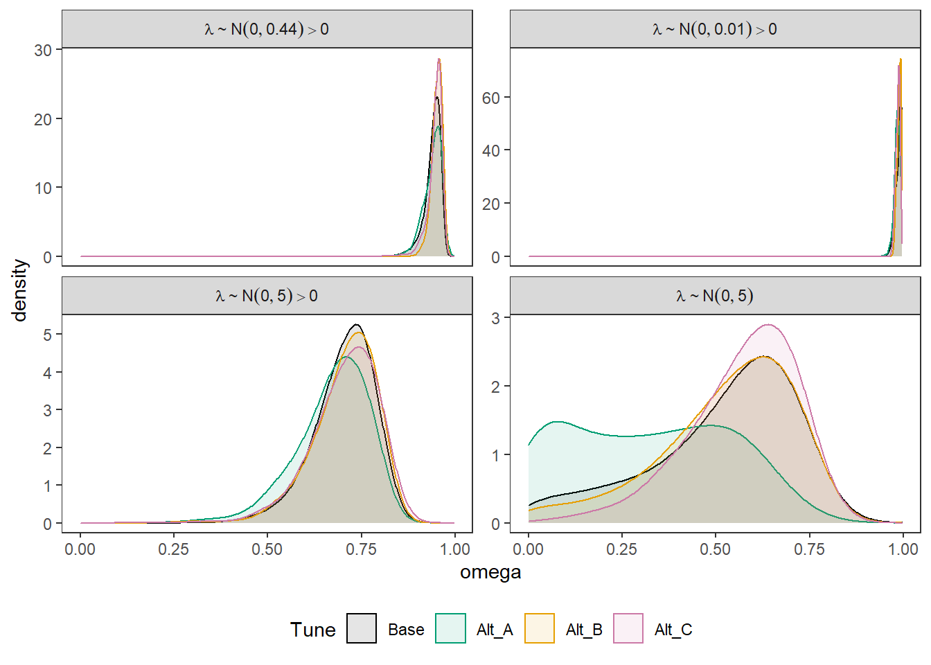
ggsave(filename = "fig/study4_prior_interactions.pdf",plot=p,width = 7, height=4,units="in")
ggsave(filename = "fig/study4_prior_interactions.png",plot=p,width = 7, height=4,units="in")
Comparing Response Probabilities
prior_lambda_base <- data.frame(
  Base = fit.base_prior$BUGSoutput$sims.matrix[,"omega[109,1,2]"],
  Alt_A = fit.base_alt_a$BUGSoutput$sims.matrix[,"omega[109,1,2]"],
  Alt_B = fit.base_alt_b$BUGSoutput$sims.matrix[,"omega[109,1,2]"],
  Alt_C = fit.base_alt_c$BUGSoutput$sims.matrix[,"omega[109,1,2]"]
)
prior_lambda_alt_a <- data.frame(
  Base = fit.alt_a_base$BUGSoutput$sims.matrix[,"omega[109,1,2]"],
  Alt_A = fit.alt_a_alt_a$BUGSoutput$sims.matrix[,"omega[109,1,2]"],
  Alt_B = fit.alt_a_alt_b$BUGSoutput$sims.matrix[,"omega[109,1,2]"],
  Alt_C = fit.alt_a_alt_c$BUGSoutput$sims.matrix[,"omega[109,1,2]"]
)
prior_lambda_alt_b <- data.frame(
  Base = fit.alt_b_base$BUGSoutput$sims.matrix[,"omega[109,1,2]"],
  Alt_A = fit.alt_b_alt_a$BUGSoutput$sims.matrix[,"omega[109,1,2]"],
  Alt_B = fit.alt_b_alt_b$BUGSoutput$sims.matrix[,"omega[109,1,2]"],
  Alt_C = fit.alt_b_alt_c$BUGSoutput$sims.matrix[,"omega[109,1,2]"]
)
prior_lambda_alt_c <- data.frame(
  Base = fit.alt_c_base$BUGSoutput$sims.matrix[,"omega[109,1,2]"],
  Alt_A = fit.alt_c_alt_a$BUGSoutput$sims.matrix[,"omega[109,1,2]"],
  Alt_B = fit.alt_c_alt_b$BUGSoutput$sims.matrix[,"omega[109,1,2]"],
  Alt_C = fit.alt_c_alt_c$BUGSoutput$sims.matrix[,"omega[109,1,2]"]
)

plot.post.base <- prior_lambda_base %>%
  pivot_longer(
    cols=everything(),
    names_to="Tune",
    values_to="omega"
  ) %>%
  mutate(
    Tune = factor(Tune, levels=c("Base", "Alt_A", "Alt_B", "Alt_C")),
    Lambda = "Base"
  )
plot.post.a <- prior_lambda_alt_a %>%
  pivot_longer(
    cols=everything(),
    names_to="Tune",
    values_to="omega"
  ) %>%
  mutate(
    Tune = factor(Tune, levels=c("Base", "Alt_A", "Alt_B", "Alt_C")),
    Lambda = "Alt_A"
  )
plot.post.b <- prior_lambda_alt_b %>%
  pivot_longer(
    cols=everything(),
    names_to="Tune",
    values_to="omega"
  ) %>%
  mutate(
    Tune = factor(Tune, levels=c("Base", "Alt_A", "Alt_B", "Alt_C")),
    Lambda = "Alt_B"
  )
plot.post.c <- prior_lambda_alt_c %>%
  pivot_longer(
    cols=everything(),
    names_to="Tune",
    values_to="omega"
  ) %>%
  mutate(
    Tune = factor(Tune, levels=c("Base", "Alt_A", "Alt_B", "Alt_C")),
    Lambda = "Alt_C"
  )
cols=c("Base"="black", "Alt_A"="#009e73", "Alt_B"="#E69F00", "Alt_C"="#CC79A7")#,"Alt_D"="#56B4E9","Alt_E"="#d55e00","Alt_F"="#f0e442") #"#56B4E9", "#E69F00" "#CC79A7", "#d55e00", "#f0e442, " #0072b2"

# joint prior and post samples
#plot.prior$type="Prior"
#plot.post$type="Post"
plot.dat <- full_join(plot.post.base, plot.post.a) %>%
  full_join(plot.post.b) %>%
  full_join(plot.post.c) %>%
  mutate(
    Lambda = factor(Lambda,
                    levels=c("Base", "Alt_A", "Alt_B", "Alt_C"),
                    labels=c("lambda%~%N(list(0, 0.44))>0", "lambda%~%N(list(0, 0.01))>0", "lambda%~%N(list(0, 5))>0", "lambda%~%N(list(0, 5))"))
  )
Joining, by = c("Tune", "omega", "Lambda")
Joining, by = c("Tune", "omega", "Lambda")
Joining, by = c("Tune", "omega", "Lambda")p <- ggplot(plot.dat, aes(x=omega, color=Tune, fill=Tune))+
geom_density(adjust=2, alpha=0.1)+
scale_color_manual(values=cols, name="Tune")+
scale_fill_manual(values=cols, name="Tune")+
labs(x="Pr(y=1|id=109) {obs y = 0}")+
facet_wrap(.~Lambda, scales="free_y",
labeller = label_parsed)+
theme_bw()+
theme(
panel.grid = element_blank(),
legend.position = "bottom"
)
p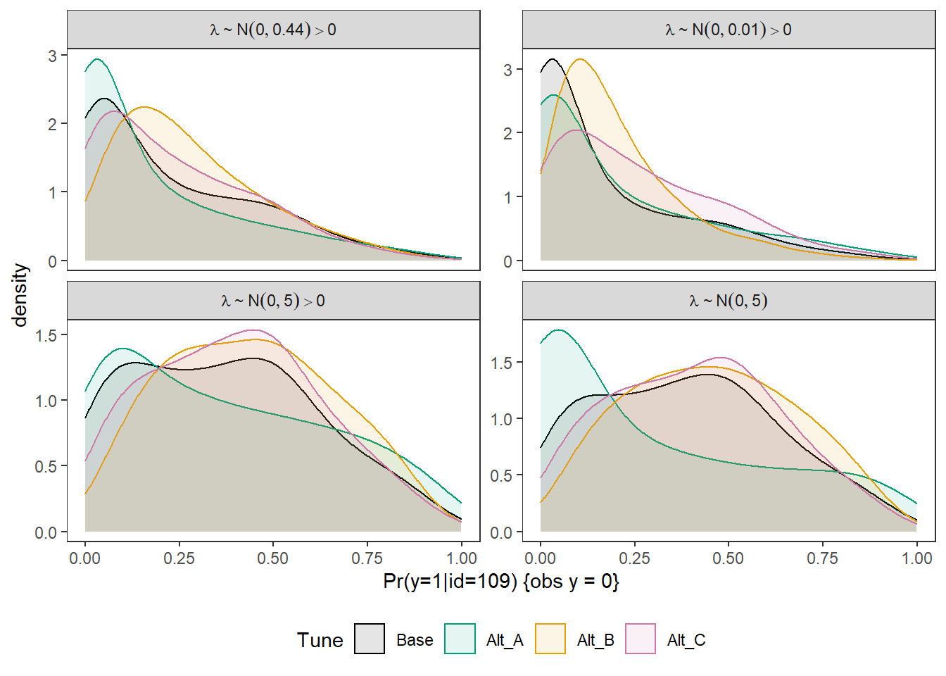
ggsave(filename = "fig/study4_prior_interactions_response_prob_id109.pdf",plot=p,width = 7, height=4,units="in")
ggsave(filename = "fig/study4_prior_interactions_response_prob_id109.png",plot=p,width = 7, height=4,units="in")
prior_lambda_base <- data.frame(
Base = fit.base_prior$BUGSoutput$sims.matrix[,"pi[109,1,2]"],
Alt_A = fit.base_alt_a$BUGSoutput$sims.matrix[,"pi[109,1,2]"],
Alt_B = fit.base_alt_b$BUGSoutput$sims.matrix[,"pi[109,1,2]"],
Alt_C = fit.base_alt_c$BUGSoutput$sims.matrix[,"pi[109,1,2]"]
)
prior_lambda_alt_a <- data.frame(
Base = fit.alt_a_base$BUGSoutput$sims.matrix[,"pi[109,1,2]"],
Alt_A = fit.alt_a_alt_a$BUGSoutput$sims.matrix[,"pi[109,1,2]"],
Alt_B = fit.alt_a_alt_b$BUGSoutput$sims.matrix[,"pi[109,1,2]"],
Alt_C = fit.alt_a_alt_c$BUGSoutput$sims.matrix[,"pi[109,1,2]"]
)
prior_lambda_alt_b <- data.frame(
Base = fit.alt_b_base$BUGSoutput$sims.matrix[,"pi[109,1,2]"],
Alt_A = fit.alt_b_alt_a$BUGSoutput$sims.matrix[,"pi[109,1,2]"],
Alt_B = fit.alt_b_alt_b$BUGSoutput$sims.matrix[,"pi[109,1,2]"],
Alt_C = fit.alt_b_alt_c$BUGSoutput$sims.matrix[,"pi[109,1,2]"]
)
prior_lambda_alt_c <- data.frame(
Base = fit.alt_c_base$BUGSoutput$sims.matrix[,"pi[109,1,2]"],
Alt_A = fit.alt_c_alt_a$BUGSoutput$sims.matrix[,"pi[109,1,2]"],
Alt_B = fit.alt_c_alt_b$BUGSoutput$sims.matrix[,"pi[109,1,2]"],
Alt_C = fit.alt_c_alt_c$BUGSoutput$sims.matrix[,"pi[109,1,2]"]
)
plot.post.base <- prior_lambda_base %>%
pivot_longer(
cols=everything(),
names_to="Tune",
values_to="pi"
) %>%
mutate(
Tune = factor(Tune, levels=c("Base", "Alt_A", "Alt_B", "Alt_C")),
Lambda = "Base"
)
plot.post.a <- prior_lambda_alt_a %>%
pivot_longer(
cols=everything(),
names_to="Tune",
values_to="pi"
) %>%
mutate(
Tune = factor(Tune, levels=c("Base", "Alt_A", "Alt_B", "Alt_C")),
Lambda = "Alt_A"
)
plot.post.b <- prior_lambda_alt_b %>%
pivot_longer(
cols=everything(),
names_to="Tune",
values_to="pi"
) %>%
mutate(
Tune = factor(Tune, levels=c("Base", "Alt_A", "Alt_B", "Alt_C")),
Lambda = "Alt_B"
)
plot.post.c <- prior_lambda_alt_c %>%
pivot_longer(
cols=everything(),
names_to="Tune",
values_to="pi"
) %>%
mutate(
Tune = factor(Tune, levels=c("Base", "Alt_A", "Alt_B", "Alt_C")),
Lambda = "Alt_C"
)
cols=c("Base"="black", "Alt_A"="#009e73", "Alt_B"="#E69F00", "Alt_C"="#CC79A7")#,"Alt_D"="#56B4E9","Alt_E"="#d55e00","Alt_F"="#f0e442") #"#56B4E9", "#E69F00" "#CC79A7", "#d55e00", "#f0e442, " #0072b2"
# joint prior and post samples
#plot.prior$type="Prior"
#plot.post$type="Post"
plot.dat <- full_join(plot.post.base, plot.post.a) %>%
full_join(plot.post.b) %>%
full_join(plot.post.c) %>%
mutate(
Lambda = factor(Lambda,
levels=c("Base", "Alt_A", "Alt_B", "Alt_C"),
labels=c("lambda%~%N(list(0, 0.44))>0", "lambda%~%N(list(0, 0.01))>0", "lambda%~%N(list(0, 5))>0", "lambda%~%N(list(0, 5))"))
)Joining, by = c("Tune", "pi", "Lambda")
Joining, by = c("Tune", "pi", "Lambda")
Joining, by = c("Tune", "pi", "Lambda")p <- ggplot(plot.dat, aes(x=pi, color=Tune, fill=Tune))+
geom_density(adjust=2, alpha=0.1)+
scale_color_manual(values=cols, name="Tune")+
scale_fill_manual(values=cols, name="Tune")+
labs(x="Pr(nu=1|id=109) {obs y = 0}")+
facet_wrap(.~Lambda, scales="free_y",
labeller = label_parsed)+
theme_bw()+
theme(
panel.grid = element_blank(),
legend.position = "bottom"
)
p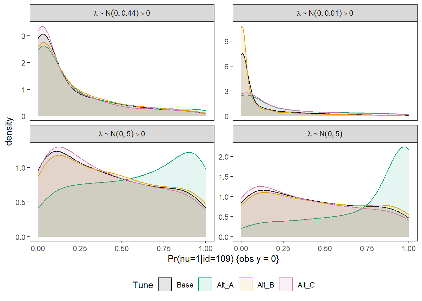
ggsave(filename = "fig/study4_prior_interactions_latent_response_prob_id109.pdf",plot=p,width = 7, height=4,units="in")
ggsave(filename = "fig/study4_prior_interactions_latent_response_prob_id109.png",plot=p,width = 7, height=4,units="in")
sessionInfo()R version 4.0.5 (2021-03-31)
Platform: x86_64-w64-mingw32/x64 (64-bit)
Running under: Windows 10 x64 (build 22000)
Matrix products: default
locale:
[1] LC_COLLATE=English_United States.1252
[2] LC_CTYPE=English_United States.1252
[3] LC_MONETARY=English_United States.1252
[4] LC_NUMERIC=C
[5] LC_TIME=English_United States.1252
attached base packages:
[1] stats graphics grDevices utils datasets methods base
other attached packages:
[1] car_3.0-10 carData_3.0-4 mvtnorm_1.1-1
[4] LaplacesDemon_16.1.4 runjags_2.2.0-2 lme4_1.1-26
[7] Matrix_1.3-2 sirt_3.9-4 R2jags_0.6-1
[10] rjags_4-12 eRm_1.0-2 diffIRT_1.5
[13] statmod_1.4.35 xtable_1.8-4 kableExtra_1.3.4
[16] lavaan_0.6-7 polycor_0.7-10 bayesplot_1.8.0
[19] ggmcmc_1.5.1.1 coda_0.19-4 data.table_1.14.0
[22] patchwork_1.1.1 forcats_0.5.1 stringr_1.4.0
[25] dplyr_1.0.5 purrr_0.3.4 readr_1.4.0
[28] tidyr_1.1.3 tibble_3.1.0 ggplot2_3.3.5
[31] tidyverse_1.3.0 workflowr_1.6.2
loaded via a namespace (and not attached):
[1] minqa_1.2.4 TAM_3.5-19 colorspace_2.0-0 rio_0.5.26
[5] ellipsis_0.3.1 ggridges_0.5.3 rprojroot_2.0.2 fs_1.5.0
[9] rstudioapi_0.13 farver_2.1.0 fansi_0.4.2 lubridate_1.7.10
[13] xml2_1.3.2 splines_4.0.5 mnormt_2.0.2 knitr_1.31
[17] jsonlite_1.7.2 nloptr_1.2.2.2 broom_0.7.5 dbplyr_2.1.0
[21] compiler_4.0.5 httr_1.4.2 backports_1.2.1 assertthat_0.2.1
[25] cli_2.3.1 later_1.1.0.1 htmltools_0.5.1.1 tools_4.0.5
[29] gtable_0.3.0 glue_1.4.2 Rcpp_1.0.7 cellranger_1.1.0
[33] jquerylib_0.1.3 vctrs_0.3.6 svglite_2.0.0 nlme_3.1-152
[37] psych_2.0.12 xfun_0.21 ps_1.6.0 openxlsx_4.2.3
[41] rvest_1.0.0 lifecycle_1.0.0 MASS_7.3-53.1 scales_1.1.1
[45] ragg_1.1.1 hms_1.0.0 promises_1.2.0.1 parallel_4.0.5
[49] RColorBrewer_1.1-2 curl_4.3 yaml_2.2.1 sass_0.3.1
[53] reshape_0.8.8 stringi_1.5.3 highr_0.8 zip_2.1.1
[57] boot_1.3-27 rlang_0.4.10 pkgconfig_2.0.3 systemfonts_1.0.1
[61] evaluate_0.14 lattice_0.20-41 labeling_0.4.2 tidyselect_1.1.0
[65] GGally_2.1.1 plyr_1.8.6 magrittr_2.0.1 R6_2.5.0
[69] generics_0.1.0 DBI_1.1.1 foreign_0.8-81 pillar_1.5.1
[73] haven_2.3.1 withr_2.4.1 abind_1.4-5 modelr_0.1.8
[77] crayon_1.4.1 utf8_1.1.4 tmvnsim_1.0-2 rmarkdown_2.7
[81] grid_4.0.5 readxl_1.3.1 CDM_7.5-15 pbivnorm_0.6.0
[85] git2r_0.28.0 reprex_1.0.0 digest_0.6.27 webshot_0.5.2
[89] httpuv_1.5.5 textshaping_0.3.1 stats4_4.0.5 munsell_0.5.0
[93] viridisLite_0.3.0 bslib_0.2.4 R2WinBUGS_2.1-21