Study 4: Extroversion Data Analysis
Full Model Prior-Posterior Sensitivity Part 1
R. Noah Padgett
2022-01-17
Last updated: 2022-02-15
Checks: 4 2
Knit directory: Padgett-Dissertation/
This reproducible R Markdown analysis was created with workflowr (version 1.6.2). The Checks tab describes the reproducibility checks that were applied when the results were created. The Past versions tab lists the development history.
Great job! The global environment was empty. Objects defined in the global environment can affect the analysis in your R Markdown file in unknown ways. For reproduciblity it’s best to always run the code in an empty environment.
The command set.seed(20210401) was run prior to running the code in the R Markdown file. Setting a seed ensures that any results that rely on randomness, e.g. subsampling or permutations, are reproducible.
Great job! Recording the operating system, R version, and package versions is critical for reproducibility.
- base-base
- model4-alt-a-alt-a
- model4-alt-a-alt-b
- model4-alt-a-alt-c
- model4-alt-a-alt-d
- model4-alt-a-base
- model4-alt-b-alt-a
- model4-alt-b-alt-b
- model4-alt-b-alt-c
- model4-alt-b-alt-d
- model4-alt-b-base
- model4-alt-c-alt-a
- model4-alt-c-alt-b
- model4-alt-c-alt-c
- model4-alt-c-alt-d
- model4-alt-c-base
- model4-alt-d-alt-a
- model4-alt-d-alt-b
- model4-alt-d-alt-c
- model4-alt-d-alt-d
- model4-alt-d-base
- model4-alt-e-alt-a
- model4-alt-e-alt-b
- model4-alt-e-alt-c
- model4-alt-e-alt-d
- model4-alt-e-base
- model4-alt-f-alt-a
- model4-alt-f-alt-b
- model4-alt-f-alt-c
- model4-alt-f-alt-d
- model4-alt-f-base
- model4-alt-g-alt-a
- model4-alt-g-alt-b
- model4-alt-g-alt-c
- model4-alt-g-alt-d
- model4-alt-g-base
- model4-base-alt-a
- model4-base-alt-b
- model4-base-alt-c
- model4-base-alt-d
- model4-code
- model4-post-prior-comp
- model4-spec-alt-a
- model4-spec-alt-b
- model4-spec-alt-c
- model4-spec-alt-d
- model4-spec-alt-e
- model4-spec-alt-f
- model4-spec-alt-g
- model4-spec-compare
To ensure reproducibility of the results, delete the cache directory study4_posterior_sensitivity_analysis_part4_cache and re-run the analysis. To have workflowr automatically delete the cache directory prior to building the file, set delete_cache = TRUE when running wflow_build() or wflow_publish().
Great job! Using relative paths to the files within your workflowr project makes it easier to run your code on other machines.
Tracking code development and connecting the code version to the results is critical for reproducibility. To start using Git, open the Terminal and type git init in your project directory.
This project is not being versioned with Git. To obtain the full reproducibility benefits of using workflowr, please see ?wflow_start.
# Load packages & utility functions
source("code/load_packages.R")
source("code/load_utility_functions.R")
# environment options
options(scipen = 999, digits=3)

library(diffIRT)
data("extraversion")
mydata <- na.omit(extraversion)

# model constants
# Save parameters
jags.params <- c("tau",
                 "lambda","lambda.std",
                 "theta",
                 "icept",
                 "prec",
                 "prec.s",
                 "sigma.ts",
                 "rho",
                 "reli.omega")
#data
jags.data <- list(
  y = mydata[,1:10],
  lrt = mydata[,11:20],
  N = nrow(mydata),
  nit = 10,
  ncat = 2
)


NBURN = 5000
NITER = 10000
Model 4: Full IFA with Misclassification
The code below contains the specification of the full model that has been used throughout this project.
cat(read_file(paste0(w.d, "/code/study_4/model_4.txt")))model {
### Model
for(p in 1:N){
for(i in 1:nit){
# data model
y[p,i] ~ dbern(omega[p,i,2])
# LRV
ystar[p,i] ~ dnorm(lambda[i]*eta[p], 1)
# Pr(nu = 2)
pi[p,i,2] = phi(ystar[p,i] - tau[i,1])
# Pr(nu = 1)
pi[p,i,1] = 1 - phi(ystar[p,i] - tau[i,1])
# log-RT model
dev[p,i]<-lambda[i]*(eta[p] - tau[i,1])
mu.lrt[p,i] <- icept[i] - speed[p] - rho * abs(dev[p,i])
lrt[p,i] ~ dnorm(mu.lrt[p,i], prec[i])
# MISCLASSIFICATION MODEL
for(c in 1:ncat){
# generate informative prior for misclassificaiton
# parameters based on RT
for(ct in 1:ncat){
alpha[p,i,ct,c] <- ifelse(c == ct,
ilogit(lrt[p,i]),
(1/(ncat-1))*(1-ilogit(lrt[p,i]))
)
}
# sample misclassification parameters using the informative priors
gamma[p,i,c,1:ncat] ~ ddirch(alpha[p,i,c,1:ncat])
# observed category prob (Pr(y=c))
omega[p,i, c] = gamma[p,i,c,1]*pi[p,i,1] +
gamma[p,i,c,2]*pi[p,i,2]
}
}
}
### Priors
# person parameters
for(p in 1:N){
eta[p] ~ dnorm(0, 1) # latent ability
speed[p]~dnorm(sigma.ts*eta[p],prec.s) # latent speed
}
sigma.ts ~ dnorm(0, 0.1)
prec.s ~ dgamma(.1,.1)
# transformations
sigma.t = pow(prec.s, -1) + pow(sigma.ts, 2) # speed variance
cor.ts = sigma.ts/(pow(sigma.t,0.5)) # LV correlation
for(i in 1:nit){
# lrt parameters
icept[i]~dnorm(0,.1)
prec[i]~dgamma(.1,.1)
# Thresholds
tau[i, 1] ~ dnorm(0.0,0.1)
# loadings
lambda[i] ~ dnorm(0, .44)T(0,)
# LRV total variance
# total variance = residual variance + fact. Var.
theta[i] = 1 + pow(lambda[i],2)
# standardized loading
lambda.std[i] = lambda[i]/pow(theta[i],0.5)
}
rho~dnorm(0,.1)I(0,)
# compute omega
lambda_sum[1] = lambda[1]
for(i in 2:nit){
#lambda_sum (sum factor loadings)
lambda_sum[i] = lambda_sum[i-1]+lambda[i]
}
reli.omega = (pow(lambda_sum[nit],2))/(pow(lambda_sum[nit],2)+nit)
}# omega simulator
prior_omega <- function(lambda, theta){
(sum(lambda)**2)/(sum(lambda)**2 + sum(theta))
}
# induced prior on omega is:
prior_lambda <- function(n){
y <- rep(-1, n)
for(i in 1:n){
while(y[i] < 0){
y[i] <- rnorm(1, 0, sqrt(1/.44))
}
}
return(y)
}
nsim=1000
sim_omega <- numeric(nsim)
for(i in 1:nsim){
lam_vec <- prior_lambda(10)
tht_vec <- rep(1, 10)
sim_omega[i] <- prior_omega(lam_vec, tht_vec)
}
prior_data <- data.frame(Base=sim_omega)
ggplot(prior_data, aes(x=Base))+
geom_density(adjust=2)+
labs(title="Induced prior on omega")+
theme_classic()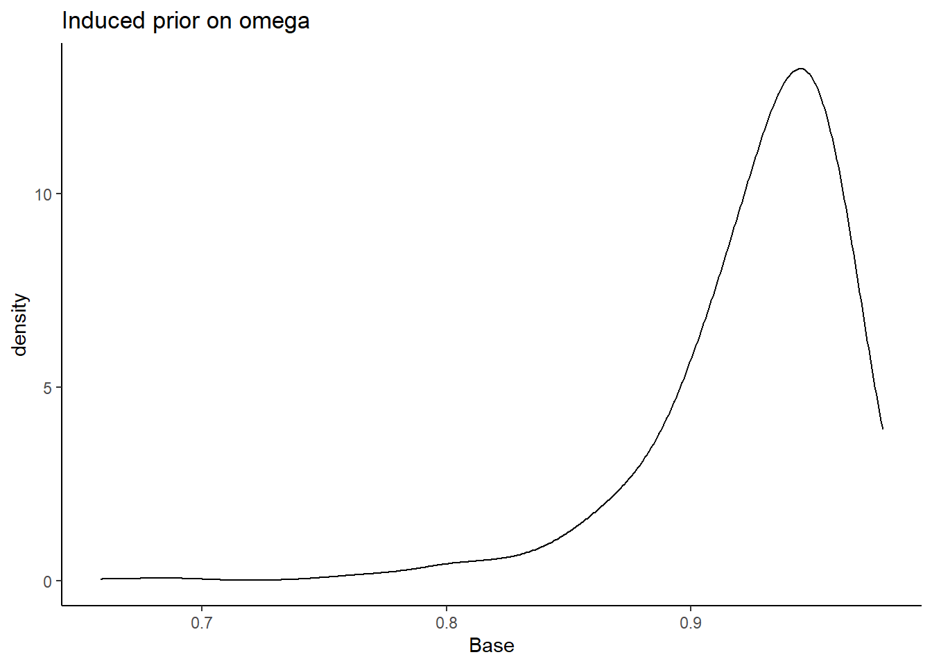
I will test the various different prior structures. The prior structure is very complex. There are many moving pieces in this posterior distribution and for this prior-posterior sensitivity analysis we will focus on the effects of prior specification on the posterior of \(\omega\) only.
The pieces are most likely to effect the posterior of \(\omega\) are the priors for the
factor loadings (\(\lambda\))
misclassification rates (\(\gamma\)) by tuning of misclassification
For each specification below, we will show the induced prior on \(\omega\).
Factor Loading Prior Alternatives
For the following investigations, the prior for the tuning parameter of misclassification rates is held constant at 1. The following major section will test how the tuning paramter incluences the results as well.
Alternative A
\[\lambda \sim N^+(0,.44) \Longrightarrow \lambda \sim N^+(0,.01)\] and remember, the variability is parameterized as the precision and not variance.
prior_lambda_A <- function(n){
  y <- rep(-1, n)
  for(i in 1:n){
    while(y[i] < 0){
      y[i] <- rnorm(1, 0, sqrt(1/.01))
    }
  }
  return(y)
}

nsim=1000
sim_omega <- numeric(nsim)
for(i in 1:nsim){
  lam_vec <- prior_lambda_A(10)
  tht_vec <- rep(1, 10)
  sim_omega[i] <- prior_omega(lam_vec, tht_vec)
}
prior_data$Alt_A <- sim_omega

ggplot(prior_data, aes(x=Alt_A))+
  geom_density(adjust=2)+
  labs(title="Induced prior on omega")+
  theme_classic()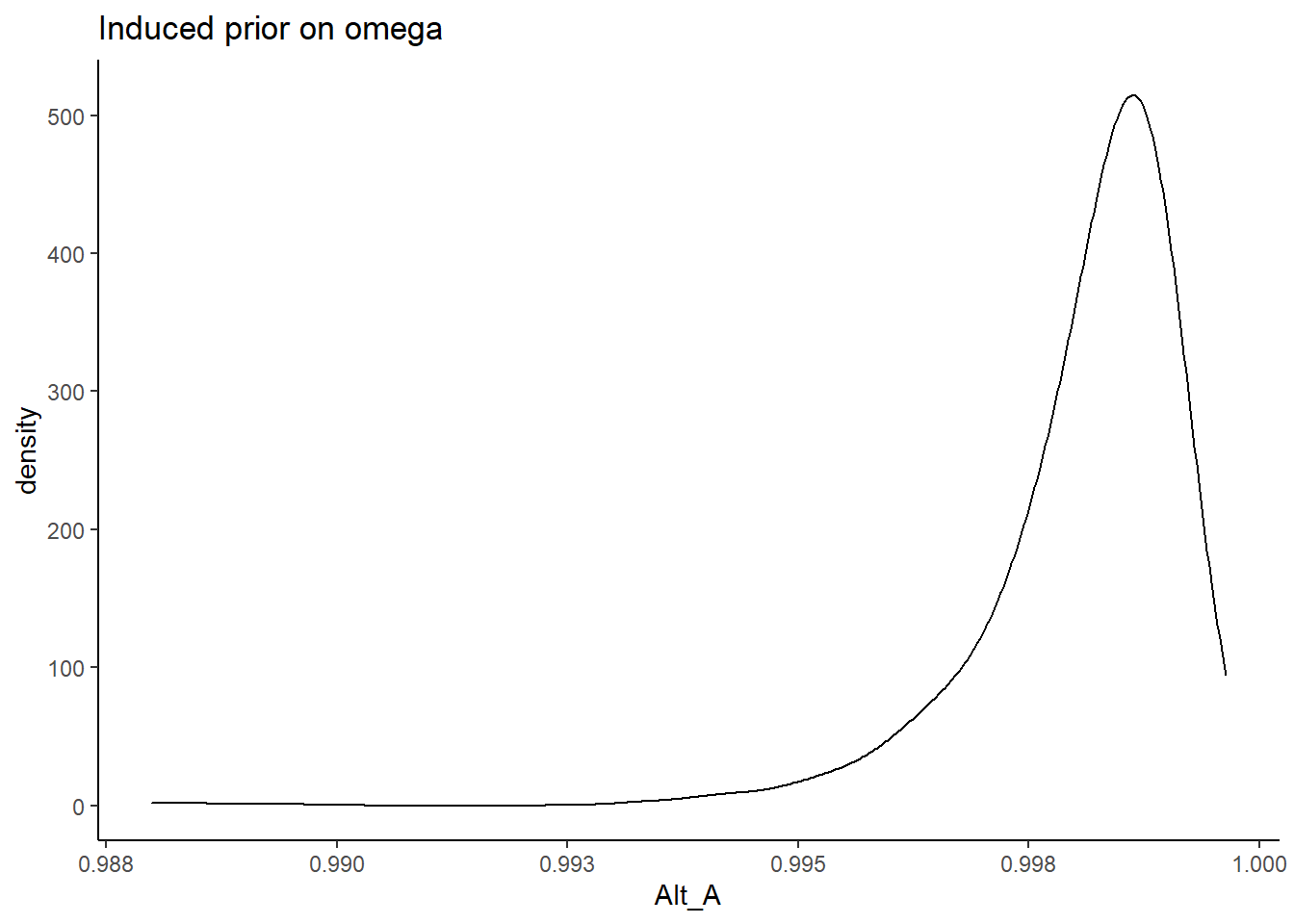
Alternative B
\[\lambda \sim N^+(0,.44) \Longrightarrow \lambda \sim N^+(0,1)\]
prior_lambda_B <- function(n){
  y <- rep(-1, n)
  for(i in 1:n){
    while(y[i] < 0){
      y[i] <- rnorm(1, 0, 1)
    }
  }
  return(y)
}

sim_omega <- numeric(nsim)
for(i in 1:nsim){
  lam_vec <- prior_lambda_B(10)
  tht_vec <- rep(1, 10)
  sim_omega[i] <- prior_omega(lam_vec, tht_vec)
}
prior_data$Alt_B <- sim_omega

ggplot(prior_data, aes(x=Alt_B))+
  geom_density(adjust=2)+
  labs(title="Induced prior on omega")+
  theme_classic()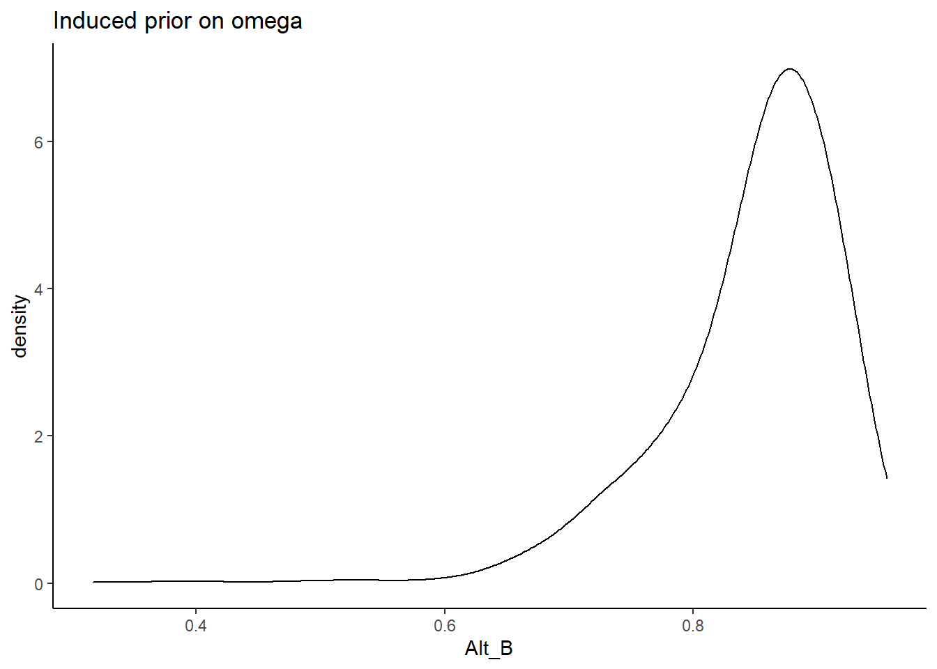
Alternative C
\[\lambda \sim N^+(0,.44) \Longrightarrow \lambda \sim N^+(0,10)\]
prior_lambda_C <- function(n){
    y <- rep(-1, n)
  for(i in 1:n){
    while(y[i] < 0){
      y[i] <- rnorm(1, 0, sqrt(1/10))
    }
  }
  return(y)
}

sim_omega <- numeric(nsim)
for(i in 1:nsim){
  lam_vec <- prior_lambda_C(10)
  tht_vec <- rep(1, 10)
  sim_omega[i] <- prior_omega(lam_vec, tht_vec)
}
prior_data$Alt_C <- sim_omega

ggplot(prior_data, aes(x=Alt_C))+
  geom_density(adjust=2)+
  labs(title="Induced prior on omega")+
  theme_classic()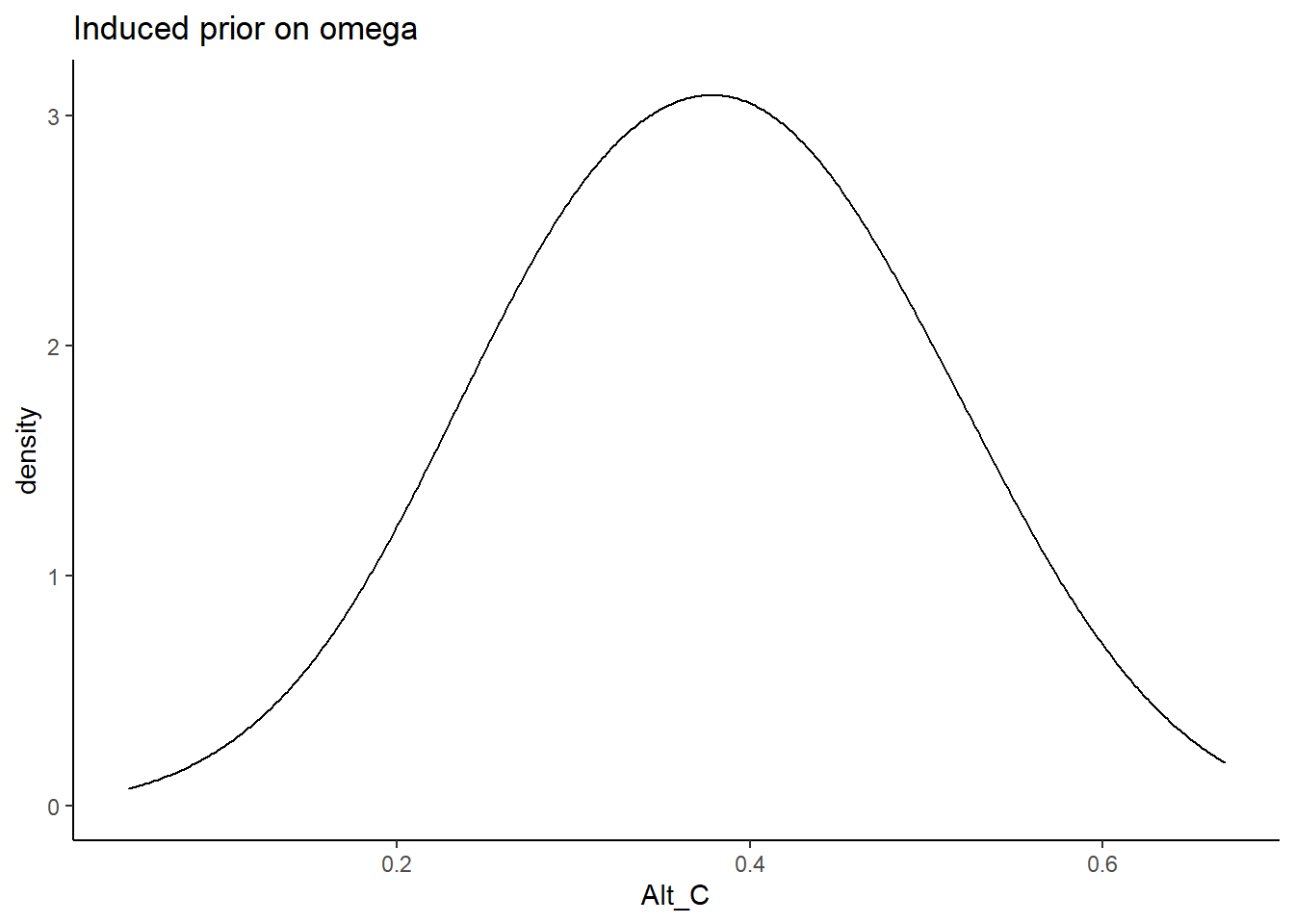
Alternative D
\[\lambda \sim N^+(0,.44) \Longrightarrow \lambda \sim N(0, 0.44)\]
prior_lambda_D <- function(n){
  rnorm(n, 0, sqrt(1/0.44))
}

sim_omega <- numeric(nsim)
for(i in 1:nsim){
  lam_vec <- prior_lambda_D(10)
  tht_vec <- rep(1, 10)
  sim_omega[i] <- prior_omega(lam_vec, tht_vec)
}
prior_data$Alt_D <- sim_omega

ggplot(prior_data, aes(x=Alt_D))+
  geom_density(adjust=2)+
  labs(title="Induced prior on omega")+
  theme_classic()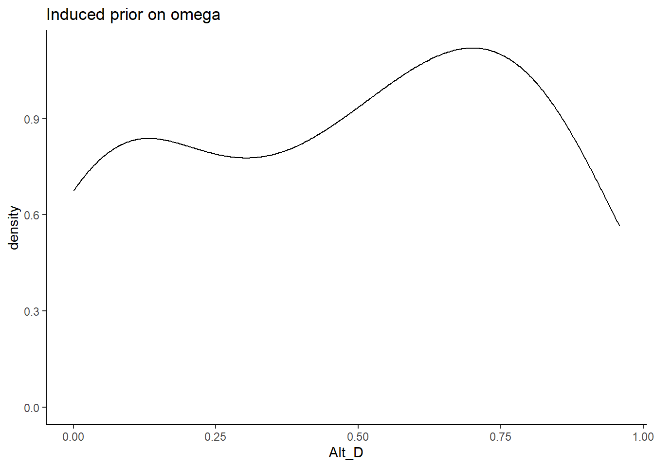
Alternative E
\[\lambda \sim N^+(0,.44) \Longrightarrow \lambda \sim N(0,0.01)\]
prior_lambda_E <- function(n){
  rnorm(n, 0, sqrt(1/0.01))
}

sim_omega <- numeric(nsim)
for(i in 1:nsim){
  lam_vec <- prior_lambda_E(10)
  tht_vec <- rep(1, 10)
  sim_omega[i] <- prior_omega(lam_vec, tht_vec)
}
prior_data$Alt_E <- sim_omega

ggplot(prior_data, aes(x=Alt_E))+
  geom_density(adjust=2)+
  labs(title="Induced prior on omega")+
  theme_classic()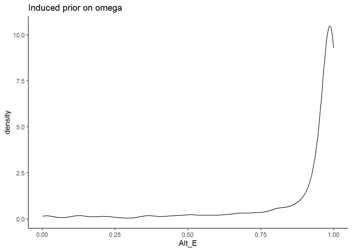
Alternative F
\[\lambda \sim N^+(0,.44) \Longrightarrow \lambda \sim N(0,1)\]
prior_lambda_F <- function(n){
  rnorm(n, 0, 1)
}

sim_omega <- numeric(nsim)
for(i in 1:nsim){
  lam_vec <- prior_lambda_F(10)
  tht_vec <- rep(1, 10)
  sim_omega[i] <- prior_omega(lam_vec, tht_vec)
}
prior_data$Alt_F <- sim_omega

ggplot(prior_data, aes(x=Alt_F))+
  geom_density(adjust=2)+
  labs(title="Induced prior on omega")+
  theme_classic()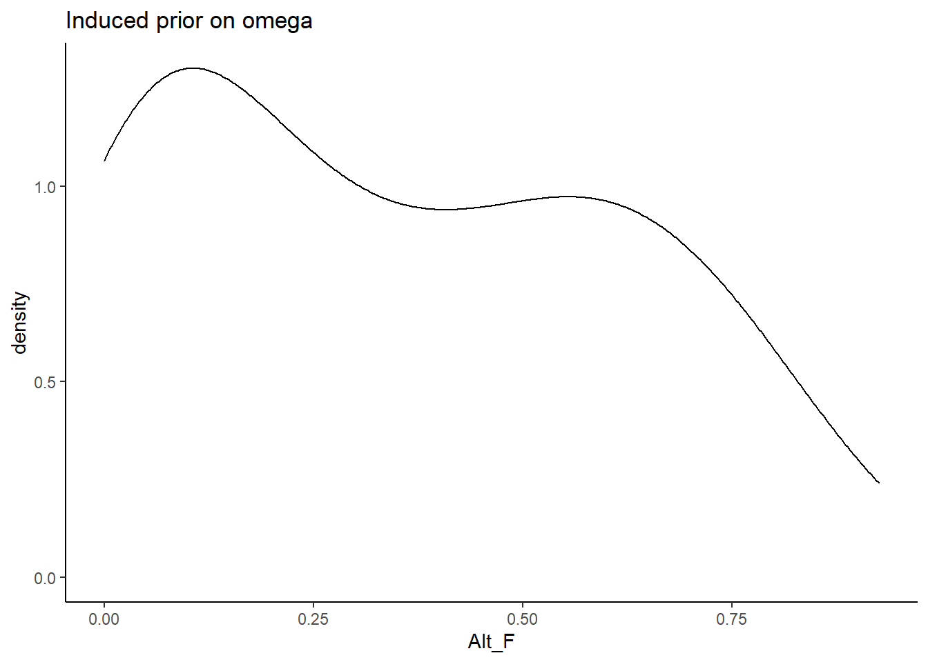
Alternative G
\[\lambda \sim N^+(0,.44) \Longrightarrow \lambda \sim N(0,10)\]
prior_lambda_G <- function(n){
  rnorm(n, 0, sqrt(1/10))
}

sim_omega <- numeric(nsim)
for(i in 1:nsim){
  lam_vec <- prior_lambda_G(10)
  tht_vec <- rep(1, 10)
  sim_omega[i] <- prior_omega(lam_vec, tht_vec)
}
prior_data$Alt_G <- sim_omega

ggplot(prior_data, aes(x=Alt_G))+
  geom_density(adjust=2)+
  labs(title="Induced prior on omega")+
  theme_classic()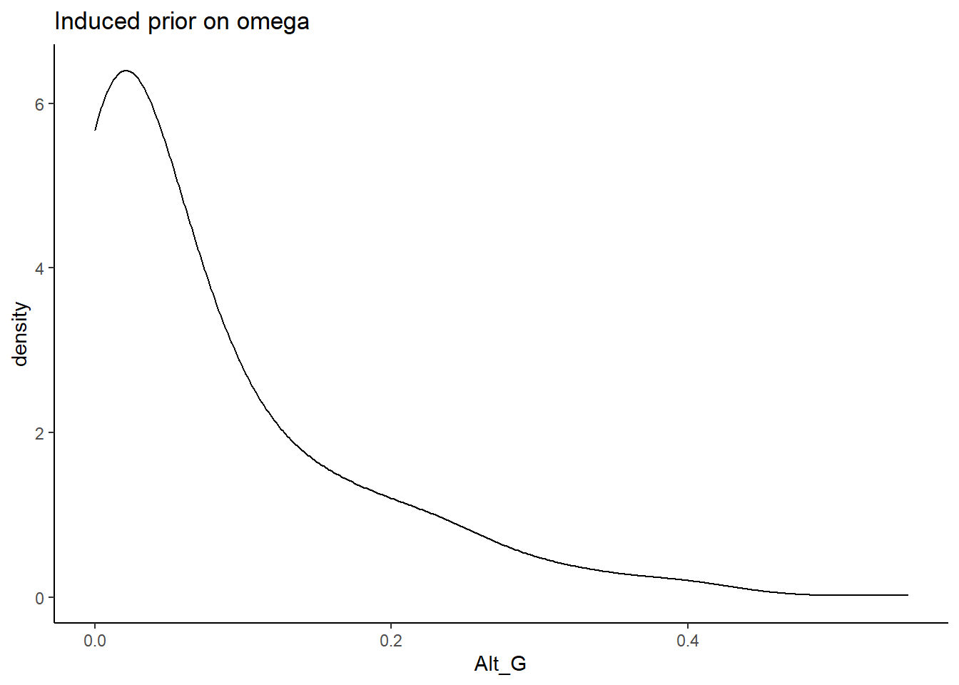
Comparing A-E
# lambda
prior_dat_lambda <- data.frame(
  Base = prior_lambda(10000),
  Alt_A = prior_lambda_A(10000),
  Alt_B = prior_lambda_B(10000),
  Alt_C = prior_lambda_C(10000),
  Alt_D = prior_lambda_D(10000),
  Alt_E = prior_lambda_E(10000),
  Alt_F = prior_lambda_F(10000),
  Alt_G = prior_lambda_G(10000)
)%>%
  pivot_longer(
    cols=everything(),
    names_to="Prior",
    values_to="lambda"
  ) %>%
  mutate(
    Prior = factor(Prior, levels=c("Base", "Alt_A", "Alt_B", "Alt_C", "Alt_D", "Alt_E", "Alt_F", "Alt_G"))
  )
cols=c("Base"="black", "Alt_A"="#009e73", "Alt_B"="#E69F00", "Alt_C"="#CC79A7","Alt_D"="#56B4E9", "Alt_E"="#f0e442", "Alt_F"="#0072b2", "Alt_G"="#d55e00") #"#56B4E9", "#E69F00" "#CC79A7", "#d55e00", "#f0e442, "  #0072b2"

p1 <- ggplot(prior_dat_lambda, aes(x=lambda, color=Prior, fill=Prior))+
  geom_density(adjust=0.1, alpha=0.1, size=1)+
  scale_color_manual(values=cols, name="Prior")+
  scale_fill_manual(values=cols, name="Prior")+
  lims(x=c(-5,5))+
  theme_bw()+
  theme(
    panel.grid = element_blank()
  )
p1
Warning: Removed 12411 rows containing non-finite values (stat_density).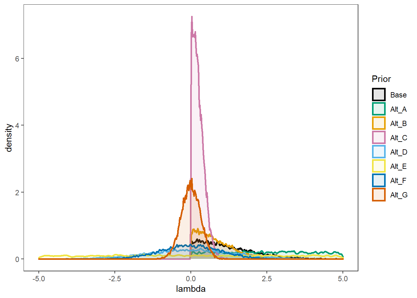
plot.prior <- prior_data %>%
  pivot_longer(
    cols=everything(),
    names_to="Prior",
    values_to="omega"
  ) %>%
  mutate(
    Prior = factor(Prior, levels=c("Base", "Alt_A", "Alt_B", "Alt_C", "Alt_D", "Alt_E", "Alt_F", "Alt_G"))
  )
cols=c("Base"="black", "Alt_A"="#009e73", "Alt_B"="#E69F00", "Alt_C"="#CC79A7","Alt_D"="#56B4E9", "Alt_E"="#f0e442", "Alt_F"="#0072b2", "Alt_G"="#d55e00") #"#56B4E9", "#E69F00" "#CC79A7", "#d55e00", "#f0e442, "  #0072b2"

p2 <- ggplot(plot.prior, aes(x=omega, color=Prior, fill=Prior))+
  geom_density(adjust=2, alpha=0.1, size=1)+
  scale_color_manual(values=cols, name="Prior")+
  scale_fill_manual(values=cols, name="Prior")+
  lims(y=c(0,20))+
  theme_bw()+
  theme(
    panel.grid = element_blank()
  )
p2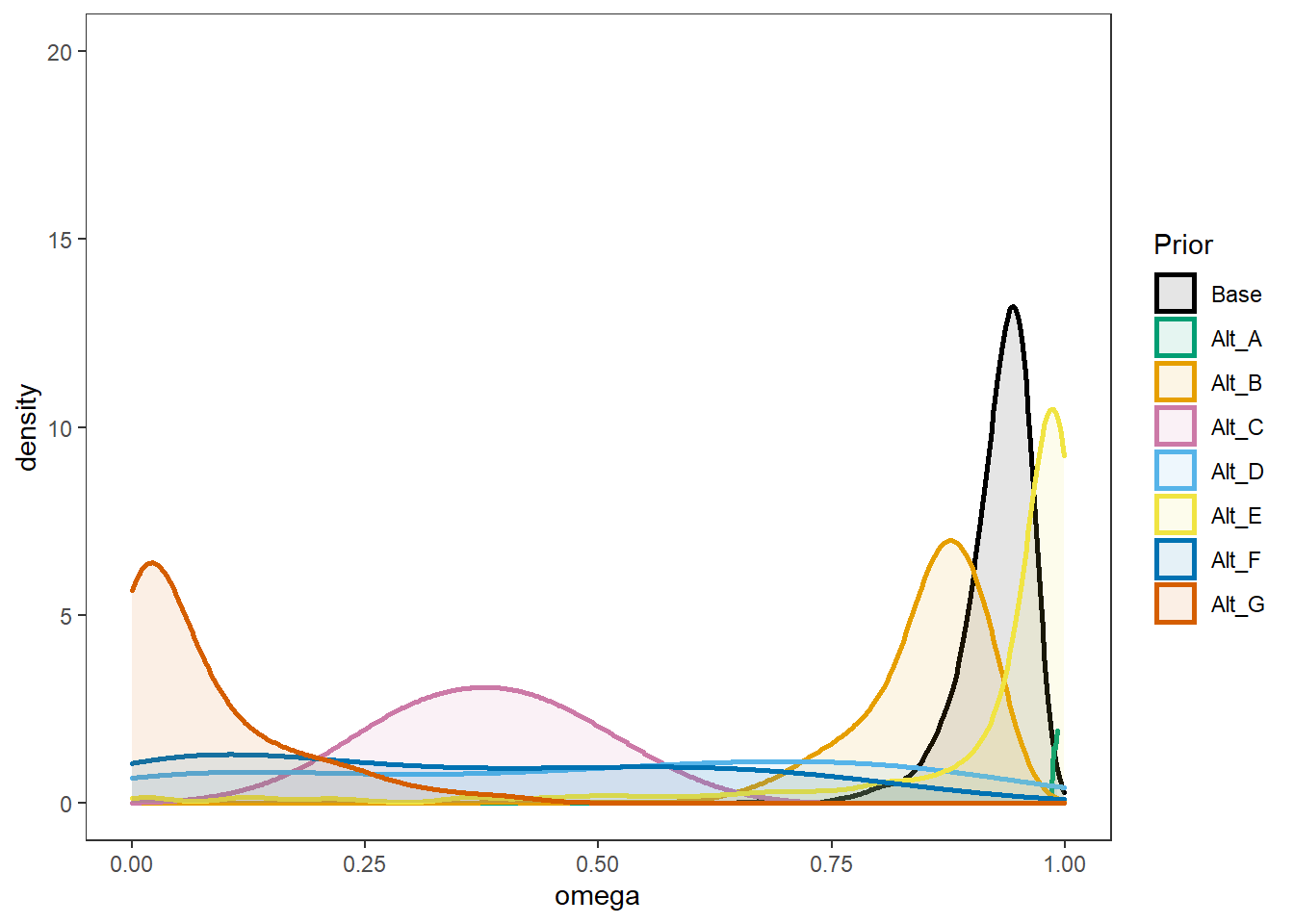
p1 + p2 + plot_layout(guides="collect")Warning: Removed 12411 rows containing non-finite values (stat_density).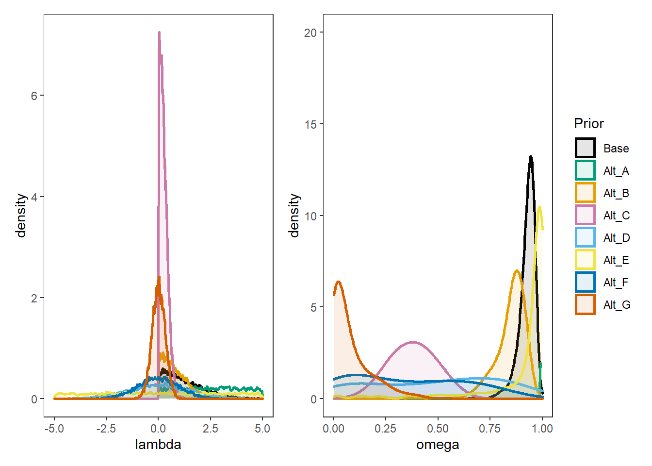
Estimate Models
Base Priors
For the base model, the priors are
\[\lambda \sim N^+(0,.44)\] \[\xi = 1\]
# Save parameters
jags.params <- c("lambda.std",
                 "reli.omega",
                 "gamma[109,1,1,1]",
                 "gamma[109,1,1,2]",
                 "gamma[109,1,2,1]",
                 "gamma[109,1,2,2]",
                 "omega[109,1,2]",
                 "pi[109,1,2]",
                 "gamma[98,1,1,1]",
                 "gamma[98,1,1,2]",
                 "gamma[98,1,2,1]",
                 "gamma[98,1,2,2]",
                 "omega[98,1,2]",
                 "pi[98,1,2]")
# initial-values
jags.inits <- function(){
    list(
      "tau"=matrix(c(-0.64, -0.09, -1.05, -1.42, -0.11, -1.29, -1.59, -1.81, -0.93, -1.11), ncol=1, nrow=10),
      "lambda"=rep(0.7,10),
      "eta"=rnorm(142),
      "speed"=rnorm(142),
      "ystar"=matrix(c(0.7*rep(rnorm(142),10)), ncol=10),
      "rho"=0.1,
      "icept"=rep(0, 10),
      "prec.s"=10,
      "prec"=rep(4, 10),
      "sigma.ts"=0.1
    )
  }
jags.data <- list(
  y = mydata[,1:10],
  lrt = mydata[,11:20],
  N = nrow(mydata),
  nit = 10,
  ncat = 2,
  xi = 1
)

# Run model
fit.base_prior <-  R2jags::jags(
  model = paste0(w.d, "/code/study_4/model_4w_xi.txt"),
  parameters.to.save = jags.params,
  inits = jags.inits,
  data = jags.data,
  n.chains = 4,
  n.burnin = NBURN,
  n.iter = NITER
)
module glm loadedCompiling model graph
Resolving undeclared variables
Allocating nodes
Graph information:
Observed stochastic nodes: 2840
Unobserved stochastic nodes: 4587
Total graph size: 45400
Initializing modelBase \(\lambda\) Prior with Alt Tune A \(\xi = 0.1\)
\[\lambda \sim N^+(0,.44)\] \[\xi = 0.1\]
jags.data <- list(
  y = mydata[,1:10],
  lrt = mydata[,11:20],
  N = nrow(mydata),
  nit = 10,
  ncat = 2,
  xi = 0.1
)

# Run model
fit.base_alt_a <-  R2jags::jags(
  model = paste0(w.d, "/code/study_4/model_4w_xi.txt"),
  parameters.to.save = jags.params,
  inits = jags.inits,
  data = jags.data,
  n.chains = 4,
  n.burnin = NBURN,
  n.iter = NITER
)
Compiling model graph
Resolving undeclared variables
Allocating nodes
Graph information:
Observed stochastic nodes: 2840
Unobserved stochastic nodes: 4587
Total graph size: 45400
Initializing modelprint(fit.base_alt_a, width=1000)Inference for Bugs model at "C:/Users/noahp/Documents/GitHub/Padgett-Dissertation/code/study_4/model_4w_xi.txt", fit using jags,
4 chains, each with 10000 iterations (first 5000 discarded), n.thin = 5
n.sims = 4000 iterations saved
mu.vect sd.vect 2.5% 25% 50% 75% 97.5% Rhat n.eff
gamma[109,1,1,1] 0.851 0.338 0.000 1.000 1.000 1.000 1.000 1.00 4000
gamma[109,1,1,2] 0.149 0.338 0.000 0.000 0.000 0.000 1.000 1.00 4000
gamma[109,1,2,1] 0.150 0.342 0.000 0.000 0.000 0.000 1.000 1.77 7
gamma[109,1,2,2] 0.850 0.342 0.000 1.000 1.000 1.000 1.000 1.25 30
gamma[98,1,1,1] 0.666 0.448 0.000 0.019 1.000 1.000 1.000 1.00 4000
gamma[98,1,1,2] 0.334 0.448 0.000 0.000 0.000 0.981 1.000 1.00 3200
gamma[98,1,2,1] 0.357 0.463 0.000 0.000 0.000 0.999 1.000 1.48 10
gamma[98,1,2,2] 0.643 0.463 0.000 0.001 1.000 1.000 1.000 1.98 7
lambda.std[1] 0.772 0.171 0.276 0.707 0.831 0.892 0.947 1.22 22
lambda.std[2] 0.850 0.111 0.554 0.815 0.880 0.925 0.967 1.22 22
lambda.std[3] 0.899 0.075 0.708 0.878 0.921 0.948 0.970 1.26 25
lambda.std[4] 0.576 0.252 0.038 0.401 0.630 0.785 0.916 1.14 30
lambda.std[5] 0.814 0.121 0.496 0.764 0.845 0.898 0.955 1.29 16
lambda.std[6] 0.505 0.246 0.039 0.308 0.534 0.721 0.879 1.00 560
lambda.std[7] 0.412 0.246 0.019 0.202 0.416 0.610 0.864 1.00 610
lambda.std[8] 0.485 0.252 0.030 0.278 0.510 0.700 0.872 1.04 72
lambda.std[9] 0.603 0.250 0.046 0.441 0.681 0.800 0.913 1.28 16
lambda.std[10] 0.761 0.202 0.146 0.703 0.836 0.900 0.946 1.34 17
omega[109,1,2] 0.224 0.248 0.000 0.014 0.120 0.382 0.824 1.31 19
omega[98,1,2] 0.780 0.235 0.193 0.646 0.868 0.976 1.000 1.01 530
pi[109,1,2] 0.272 0.302 0.000 0.013 0.141 0.476 0.963 1.31 18
pi[98,1,2] 0.603 0.364 0.000 0.248 0.718 0.954 1.000 1.40 14
reli.omega 0.938 0.021 0.886 0.927 0.943 0.955 0.967 1.23 17
deviance 2743.862 46.630 2659.313 2711.985 2742.954 2773.882 2840.681 1.09 36
For each parameter, n.eff is a crude measure of effective sample size,
and Rhat is the potential scale reduction factor (at convergence, Rhat=1).
DIC info (using the rule, pD = var(deviance)/2)
pD = 994.6 and DIC = 3738.5
DIC is an estimate of expected predictive error (lower deviance is better).Base \(\lambda\) Prior with Alt Tune B \(\xi = 10\)
\[\lambda \sim N^+(0,.44)\] \[\xi = 10\]
jags.data <- list(
  y = mydata[,1:10],
  lrt = mydata[,11:20],
  N = nrow(mydata),
  nit = 10,
  ncat = 2,
  xi = 10
)

# Run model
fit.base_alt_b <-  R2jags::jags(
  model = paste0(w.d, "/code/study_4/model_4w_xi.txt"),
  parameters.to.save = jags.params,
  inits = jags.inits,
  data = jags.data,
  n.chains = 4,
  n.burnin = NBURN,
  n.iter = NITER
)
Compiling model graph
Resolving undeclared variables
Allocating nodes
Graph information:
Observed stochastic nodes: 2840
Unobserved stochastic nodes: 4587
Total graph size: 45400
Initializing modelprint(fit.base_alt_b, width=1000)Inference for Bugs model at "C:/Users/noahp/Documents/GitHub/Padgett-Dissertation/code/study_4/model_4w_xi.txt", fit using jags,
4 chains, each with 10000 iterations (first 5000 discarded), n.thin = 5
n.sims = 4000 iterations saved
mu.vect sd.vect 2.5% 25% 50% 75% 97.5% Rhat n.eff
gamma[109,1,1,1] 0.852 0.105 0.590 0.795 0.873 0.932 0.987 1.00 4000
gamma[109,1,1,2] 0.148 0.105 0.013 0.068 0.127 0.205 0.410 1.00 4000
gamma[109,1,2,1] 0.142 0.103 0.011 0.062 0.118 0.198 0.397 1.00 3400
gamma[109,1,2,2] 0.858 0.103 0.603 0.802 0.882 0.938 0.989 1.01 550
gamma[98,1,1,1] 0.668 0.142 0.357 0.574 0.681 0.775 0.903 1.00 2600
gamma[98,1,1,2] 0.332 0.142 0.097 0.225 0.319 0.426 0.643 1.00 3600
gamma[98,1,2,1] 0.356 0.144 0.107 0.251 0.343 0.454 0.657 1.00 4000
gamma[98,1,2,2] 0.644 0.144 0.343 0.546 0.657 0.749 0.893 1.00 4000
lambda.std[1] 0.786 0.138 0.410 0.732 0.824 0.883 0.945 1.08 99
lambda.std[2] 0.852 0.119 0.527 0.809 0.889 0.935 0.976 1.03 200
lambda.std[3] 0.905 0.058 0.760 0.887 0.920 0.941 0.965 1.09 61
lambda.std[4] 0.711 0.226 0.114 0.601 0.793 0.881 0.946 1.09 46
lambda.std[5] 0.637 0.219 0.137 0.496 0.690 0.810 0.934 1.05 76
lambda.std[6] 0.476 0.243 0.034 0.281 0.497 0.681 0.872 1.03 88
lambda.std[7] 0.494 0.242 0.035 0.298 0.529 0.701 0.865 1.01 280
lambda.std[8] 0.430 0.246 0.021 0.217 0.434 0.644 0.833 1.00 560
lambda.std[9] 0.680 0.177 0.228 0.593 0.724 0.812 0.902 1.04 170
lambda.std[10] 0.887 0.072 0.699 0.863 0.904 0.935 0.967 1.06 64
omega[109,1,2] 0.268 0.187 0.024 0.123 0.224 0.371 0.718 1.01 410
omega[98,1,2] 0.468 0.142 0.188 0.371 0.478 0.553 0.756 1.00 1300
pi[109,1,2] 0.184 0.242 0.000 0.006 0.069 0.280 0.861 1.01 300
pi[98,1,2] 0.322 0.328 0.000 0.019 0.202 0.584 0.981 1.10 150
reli.omega 0.943 0.020 0.894 0.933 0.947 0.959 0.971 1.06 59
deviance 3572.185 33.965 3504.143 3549.780 3572.593 3594.369 3639.753 1.04 73
For each parameter, n.eff is a crude measure of effective sample size,
and Rhat is the potential scale reduction factor (at convergence, Rhat=1).
DIC info (using the rule, pD = var(deviance)/2)
pD = 553.2 and DIC = 4125.3
DIC is an estimate of expected predictive error (lower deviance is better).Base \(\lambda\) Prior with Alt Tune C \(\xi U(0.5,1.5)\)
\[\lambda \sim N^+(0,.44)\] \[\xi \sim Uniform(0.5,1.5)\]
jags.params <- c("lambda.std",
                 "reli.omega",
                 "gamma[109,1,1,1]",
                 "gamma[109,1,1,2]",
                 "gamma[109,1,2,1]",
                 "gamma[109,1,2,2]",
                 "omega[109,1,2]",
                 "pi[109,1,2]",
                 "gamma[98,1,1,1]",
                 "gamma[98,1,1,2]",
                 "gamma[98,1,2,1]",
                 "gamma[98,1,2,2]",
                 "omega[98,1,2]",
                 "pi[98,1,2]",
                 "xi")

jags.data <- list(
  y = mydata[,1:10],
  lrt = mydata[,11:20],
  N = nrow(mydata),
  nit = 10,
  ncat = 2
)

# Run model
fit.base_alt_c <-  R2jags::jags(
  model = paste0(w.d, "/code/study_4/model_4w_xi_uniform.txt"),
  parameters.to.save = jags.params,
  inits = jags.inits,
  data = jags.data,
  n.chains = 4,
  n.burnin = NBURN,
  n.iter = NITER
)
Compiling model graph
Resolving undeclared variables
Allocating nodes
Graph information:
Observed stochastic nodes: 2840
Unobserved stochastic nodes: 4588
Total graph size: 45401
Initializing modelprint(fit.base_alt_c, width=1000)Inference for Bugs model at "C:/Users/noahp/Documents/GitHub/Padgett-Dissertation/code/study_4/model_4w_xi_uniform.txt", fit using jags,
4 chains, each with 10000 iterations (first 5000 discarded), n.thin = 5
n.sims = 4000 iterations saved
mu.vect sd.vect 2.5% 25% 50% 75% 97.5% Rhat n.eff
gamma[109,1,1,1] 0.850 0.230 0.159 0.793 0.972 0.999 1.000 1.00 2300
gamma[109,1,1,2] 0.150 0.230 0.000 0.001 0.028 0.207 0.841 1.00 3200
gamma[109,1,2,1] 0.104 0.175 0.000 0.001 0.019 0.125 0.655 1.01 1700
gamma[109,1,2,2] 0.896 0.175 0.345 0.875 0.981 0.999 1.000 1.03 770
gamma[98,1,1,1] 0.665 0.309 0.038 0.426 0.753 0.947 1.000 1.00 4000
gamma[98,1,1,2] 0.335 0.309 0.000 0.053 0.247 0.574 0.962 1.00 4000
gamma[98,1,2,1] 0.471 0.316 0.002 0.180 0.462 0.753 0.980 1.00 4000
gamma[98,1,2,2] 0.529 0.316 0.020 0.247 0.538 0.820 0.998 1.01 840
lambda.std[1] 0.820 0.110 0.527 0.774 0.848 0.896 0.950 1.09 52
lambda.std[2] 0.822 0.149 0.411 0.769 0.874 0.924 0.967 1.08 63
lambda.std[3] 0.920 0.046 0.795 0.898 0.932 0.952 0.974 1.07 58
lambda.std[4] 0.744 0.214 0.136 0.656 0.823 0.902 0.955 1.00 1100
lambda.std[5] 0.613 0.230 0.104 0.460 0.654 0.804 0.932 1.06 57
lambda.std[6] 0.505 0.243 0.040 0.312 0.530 0.711 0.877 1.03 120
lambda.std[7] 0.481 0.243 0.034 0.287 0.503 0.689 0.856 1.04 100
lambda.std[8] 0.446 0.259 0.021 0.219 0.445 0.672 0.871 1.02 110
lambda.std[9] 0.706 0.163 0.269 0.628 0.746 0.825 0.914 1.03 130
lambda.std[10] 0.884 0.066 0.706 0.859 0.900 0.929 0.959 1.08 77
omega[109,1,2] 0.216 0.212 0.000 0.031 0.141 0.360 0.719 1.01 270
omega[98,1,2] 0.580 0.224 0.133 0.430 0.568 0.759 0.968 1.00 4000
pi[109,1,2] 0.163 0.226 0.000 0.003 0.052 0.248 0.807 1.02 160
pi[98,1,2] 0.293 0.326 0.000 0.009 0.142 0.535 0.985 1.02 700
reli.omega 0.946 0.019 0.897 0.937 0.952 0.960 0.971 1.11 35
xi 1.379 0.091 1.159 1.323 1.399 1.454 1.495 1.03 170
deviance 3292.296 44.610 3205.152 3262.394 3291.263 3321.612 3383.116 1.01 200
For each parameter, n.eff is a crude measure of effective sample size,
and Rhat is the potential scale reduction factor (at convergence, Rhat=1).
DIC info (using the rule, pD = var(deviance)/2)
pD = 980.5 and DIC = 4272.8
DIC is an estimate of expected predictive error (lower deviance is better).Base \(\lambda\) Prior with Alt Tune D \(\xi G(1,1)\)
\[\lambda \sim N^+(0,.44)\] \[\xi \sim Gamma(1,1)\]
jags.params <- c("lambda.std",
                 "reli.omega",
                 "gamma[109,1,1,1]",
                 "gamma[109,1,1,2]",
                 "gamma[109,1,2,1]",
                 "gamma[109,1,2,2]",
                 "omega[109,1,2]",
                 "pi[109,1,2]",
                 "gamma[98,1,1,1]",
                 "gamma[98,1,1,2]",
                 "gamma[98,1,2,1]",
                 "gamma[98,1,2,2]",
                 "omega[98,1,2]",
                 "pi[98,1,2]",
                 "xi")

jags.data <- list(
  y = mydata[,1:10],
  lrt = mydata[,11:20],
  N = nrow(mydata),
  nit = 10,
  ncat = 2
)

# Run model
fit.base_alt_d <-  R2jags::jags(
  model = paste0(w.d, "/code/study_4/model_4w_xi_gamma.txt"),
  parameters.to.save = jags.params,
  inits = jags.inits,
  data = jags.data,
  n.chains = 4,
  n.burnin = NBURN,
  n.iter = NITER
)
Compiling model graph
Resolving undeclared variables
Allocating nodes
Graph information:
Observed stochastic nodes: 2840
Unobserved stochastic nodes: 4588
Total graph size: 45400
Initializing modelprint(fit.base_alt_d, width=1000)Inference for Bugs model at "C:/Users/noahp/Documents/GitHub/Padgett-Dissertation/code/study_4/model_4w_xi_gamma.txt", fit using jags,
4 chains, each with 10000 iterations (first 5000 discarded), n.thin = 5
n.sims = 4000 iterations saved
mu.vect sd.vect 2.5% 25% 50% 75% 97.5% Rhat n.eff
gamma[109,1,1,1] 0.847 0.167 0.395 0.779 0.903 0.974 1.000 1.03 840
gamma[109,1,1,2] 0.153 0.167 0.000 0.026 0.097 0.221 0.605 1.07 84
gamma[109,1,2,1] 0.129 0.147 0.000 0.019 0.077 0.193 0.532 1.09 53
gamma[109,1,2,2] 0.871 0.147 0.468 0.807 0.923 0.981 1.000 1.02 820
gamma[98,1,1,1] 0.663 0.223 0.175 0.514 0.697 0.845 0.985 1.03 380
gamma[98,1,1,2] 0.337 0.223 0.015 0.155 0.303 0.486 0.825 1.05 220
gamma[98,1,2,1] 0.402 0.222 0.035 0.231 0.383 0.563 0.852 1.02 2200
gamma[98,1,2,2] 0.598 0.222 0.148 0.437 0.617 0.769 0.965 1.05 130
lambda.std[1] 0.818 0.123 0.496 0.766 0.851 0.905 0.956 1.05 360
lambda.std[2] 0.859 0.111 0.558 0.817 0.894 0.937 0.972 1.02 160
lambda.std[3] 0.912 0.063 0.756 0.892 0.927 0.951 0.975 1.12 180
lambda.std[4] 0.791 0.195 0.211 0.743 0.866 0.920 0.964 1.12 40
lambda.std[5] 0.642 0.215 0.132 0.508 0.676 0.810 0.942 1.05 79
lambda.std[6] 0.475 0.236 0.035 0.288 0.498 0.669 0.857 1.01 490
lambda.std[7] 0.435 0.243 0.020 0.232 0.443 0.632 0.866 1.02 160
lambda.std[8] 0.473 0.263 0.027 0.245 0.490 0.696 0.892 1.03 110
lambda.std[9] 0.713 0.160 0.305 0.633 0.745 0.827 0.940 1.07 68
lambda.std[10] 0.895 0.071 0.694 0.871 0.917 0.941 0.962 1.13 100
omega[109,1,2] 0.250 0.205 0.005 0.079 0.202 0.383 0.739 1.03 180
omega[98,1,2] 0.503 0.180 0.160 0.384 0.499 0.617 0.876 1.01 250
pi[109,1,2] 0.175 0.240 0.000 0.004 0.059 0.259 0.855 1.02 390
pi[98,1,2] 0.272 0.318 0.000 0.004 0.112 0.499 0.972 1.01 720
reli.omega 0.950 0.020 0.898 0.942 0.955 0.964 0.977 1.20 22
xi 4.243 2.109 2.062 2.701 3.331 5.562 9.129 2.64 5
deviance 3466.241 70.726 3330.781 3415.105 3464.109 3520.033 3596.189 1.80 7
For each parameter, n.eff is a crude measure of effective sample size,
and Rhat is the potential scale reduction factor (at convergence, Rhat=1).
DIC info (using the rule, pD = var(deviance)/2)
pD = 1258.2 and DIC = 4724.4
DIC is an estimate of expected predictive error (lower deviance is better).Alt \(\lambda\) Prior A with Base Tune \(\xi = 1\)
\[\lambda \sim N^+(0,.01)\] \[\xi = 1\]
# Save parameters
jags.params <- c("lambda.std",
                 "reli.omega",
                 "gamma[109,1,1,1]",
                 "gamma[109,1,1,2]",
                 "gamma[109,1,2,1]",
                 "gamma[109,1,2,2]",
                 "omega[109,1,2]",
                 "pi[109,1,2]",
                 "gamma[98,1,1,1]",
                 "gamma[98,1,1,2]",
                 "gamma[98,1,2,1]",
                 "gamma[98,1,2,2]",
                 "omega[98,1,2]",
                 "pi[98,1,2]")
jags.data <- list(
  y = mydata[,1:10],
  lrt = mydata[,11:20],
  N = nrow(mydata),
  nit = 10,
  ncat = 2,
  xi = 1
)

# Run model
fit.alt_a_base <-  R2jags::jags(
  model = paste0(w.d, "/code/study_4/model_4Aw_xi.txt"),
  parameters.to.save = jags.params,
  inits = jags.inits,
  data = jags.data,
  n.chains = 4,
  n.burnin = NBURN,
  n.iter = NITER
)
Compiling model graph
Resolving undeclared variables
Allocating nodes
Graph information:
Observed stochastic nodes: 2840
Unobserved stochastic nodes: 4587
Total graph size: 45400
Initializing modelprint(fit.alt_a_base, width=1000)Inference for Bugs model at "C:/Users/noahp/Documents/GitHub/Padgett-Dissertation/code/study_4/model_4Aw_xi.txt", fit using jags,
4 chains, each with 10000 iterations (first 5000 discarded), n.thin = 5
n.sims = 4000 iterations saved
mu.vect sd.vect 2.5% 25% 50% 75% 97.5% Rhat n.eff
gamma[109,1,1,1] 0.850 0.251 0.099 0.811 0.985 1.000 1.000 1.00 4000
gamma[109,1,1,2] 0.150 0.251 0.000 0.000 0.015 0.189 0.901 1.00 2600
gamma[109,1,2,1] 0.087 0.186 0.000 0.000 0.002 0.066 0.731 1.26 26
gamma[109,1,2,2] 0.913 0.186 0.269 0.934 0.998 1.000 1.000 1.05 1700
gamma[98,1,1,1] 0.673 0.327 0.017 0.407 0.797 0.973 1.000 1.00 4000
gamma[98,1,1,2] 0.327 0.327 0.000 0.027 0.203 0.593 0.983 1.00 3500
gamma[98,1,2,1] 0.557 0.327 0.002 0.262 0.606 0.863 0.994 1.02 280
gamma[98,1,2,2] 0.443 0.327 0.006 0.137 0.394 0.738 0.998 1.01 440
lambda.std[1] 0.928 0.090 0.658 0.917 0.958 0.976 0.990 1.30 37
lambda.std[2] 0.977 0.040 0.841 0.978 0.991 0.997 0.998 1.64 10
lambda.std[3] 0.952 0.044 0.841 0.944 0.965 0.977 0.989 1.38 17
lambda.std[4] 0.910 0.103 0.592 0.896 0.945 0.966 0.984 1.09 88
lambda.std[5] 0.852 0.153 0.437 0.782 0.908 0.969 0.990 1.40 12
lambda.std[6] 0.593 0.267 0.043 0.397 0.660 0.819 0.943 1.00 1300
lambda.std[7] 0.567 0.269 0.029 0.362 0.623 0.793 0.932 1.02 170
lambda.std[8] 0.574 0.278 0.033 0.349 0.629 0.819 0.944 1.09 40
lambda.std[9] 0.861 0.120 0.539 0.819 0.901 0.945 0.976 1.34 17
lambda.std[10] 0.936 0.054 0.794 0.920 0.953 0.971 0.986 1.22 29
omega[109,1,2] 0.153 0.202 0.000 0.003 0.056 0.245 0.700 1.14 87
omega[98,1,2] 0.623 0.259 0.101 0.431 0.641 0.852 0.992 1.00 4000
pi[109,1,2] 0.107 0.199 0.000 0.000 0.005 0.112 0.742 1.01 260
pi[98,1,2] 0.160 0.277 0.000 0.000 0.004 0.194 0.957 1.03 220
reli.omega 0.988 0.005 0.976 0.985 0.989 0.991 0.993 1.70 8
deviance 3138.831 46.429 3050.806 3107.466 3136.470 3169.707 3232.848 1.15 22
For each parameter, n.eff is a crude measure of effective sample size,
and Rhat is the potential scale reduction factor (at convergence, Rhat=1).
DIC info (using the rule, pD = var(deviance)/2)
pD = 926.4 and DIC = 4065.2
DIC is an estimate of expected predictive error (lower deviance is better).Alt \(\lambda\) Prior A with Alt Tune A \(\xi = 0.1\)
\[\lambda \sim N^+(0,.01)\] \[\xi = 0.1\]
jags.data <- list(
  y = mydata[,1:10],
  lrt = mydata[,11:20],
  N = nrow(mydata),
  nit = 10,
  ncat = 2,
  xi = 0.1
)

# Run model
fit.alt_a_alt_a <-  R2jags::jags(
  model = paste0(w.d, "/code/study_4/model_4Aw_xi.txt"),
  parameters.to.save = jags.params,
  inits = jags.inits,
  data = jags.data,
  n.chains = 4,
  n.burnin = NBURN,
  n.iter = NITER
)
Compiling model graph
Resolving undeclared variables
Allocating nodes
Graph information:
Observed stochastic nodes: 2840
Unobserved stochastic nodes: 4587
Total graph size: 45400
Initializing modelprint(fit.alt_a_alt_a, width=1000)Inference for Bugs model at "C:/Users/noahp/Documents/GitHub/Padgett-Dissertation/code/study_4/model_4Aw_xi.txt", fit using jags,
4 chains, each with 10000 iterations (first 5000 discarded), n.thin = 5
n.sims = 4000 iterations saved
mu.vect sd.vect 2.5% 25% 50% 75% 97.5% Rhat n.eff
gamma[109,1,1,1] 0.843 0.348 0.000 1.000 1.000 1.000 1.000 1.01 2100
gamma[109,1,1,2] 0.157 0.348 0.000 0.000 0.000 0.000 1.000 1.00 4000
gamma[109,1,2,1] 0.130 0.318 0.000 0.000 0.000 0.000 1.000 3.72 5
gamma[109,1,2,2] 0.870 0.318 0.000 1.000 1.000 1.000 1.000 1.49 15
gamma[98,1,1,1] 0.669 0.449 0.000 0.015 1.000 1.000 1.000 1.00 3800
gamma[98,1,1,2] 0.331 0.449 0.000 0.000 0.000 0.985 1.000 1.00 4000
gamma[98,1,2,1] 0.362 0.458 0.000 0.000 0.003 0.998 1.000 1.28 15
gamma[98,1,2,2] 0.638 0.458 0.000 0.002 0.997 1.000 1.000 1.21 24
lambda.std[1] 0.833 0.138 0.448 0.775 0.866 0.937 0.978 1.33 14
lambda.std[2] 0.968 0.033 0.877 0.960 0.978 0.990 0.995 1.25 17
lambda.std[3] 0.939 0.062 0.750 0.925 0.959 0.977 0.990 1.38 15
lambda.std[4] 0.553 0.264 0.037 0.356 0.588 0.776 0.935 1.10 34
lambda.std[5] 0.851 0.154 0.435 0.797 0.908 0.961 0.991 1.66 9
lambda.std[6] 0.650 0.256 0.068 0.483 0.725 0.863 0.948 1.07 57
lambda.std[7] 0.590 0.286 0.039 0.347 0.670 0.846 0.942 1.10 33
lambda.std[8] 0.611 0.280 0.041 0.397 0.690 0.857 0.945 1.11 32
lambda.std[9] 0.785 0.223 0.108 0.727 0.880 0.929 0.970 1.62 10
lambda.std[10] 0.853 0.185 0.248 0.832 0.926 0.962 0.990 1.24 23
omega[109,1,2] 0.291 0.275 0.000 0.034 0.212 0.506 0.883 1.12 37
omega[98,1,2] 0.759 0.245 0.162 0.597 0.840 0.972 1.000 1.02 180
pi[109,1,2] 0.332 0.312 0.000 0.036 0.246 0.581 0.985 1.11 43
pi[98,1,2] 0.618 0.353 0.001 0.305 0.725 0.954 1.000 1.11 81
reli.omega 0.974 0.019 0.924 0.969 0.980 0.987 0.991 1.89 7
deviance 2690.927 44.285 2608.441 2660.855 2689.680 2720.160 2780.776 1.20 17
For each parameter, n.eff is a crude measure of effective sample size,
and Rhat is the potential scale reduction factor (at convergence, Rhat=1).
DIC info (using the rule, pD = var(deviance)/2)
pD = 803.5 and DIC = 3494.4
DIC is an estimate of expected predictive error (lower deviance is better).Alt \(\lambda\) Prior A with Alt Tune B \(\xi = 10\)
\[\lambda \sim N^+(0,.01)\] \[\xi = 10\]
jags.data <- list(
  y = mydata[,1:10],
  lrt = mydata[,11:20],
  N = nrow(mydata),
  nit = 10,
  ncat = 2,
  xi = 10
)

# Run model
fit.alt_a_alt_b <-  R2jags::jags(
  model = paste0(w.d, "/code/study_4/model_4Aw_xi.txt"),
  parameters.to.save = jags.params,
  inits = jags.inits,
  data = jags.data,
  n.chains = 4,
  n.burnin = NBURN,
  n.iter = NITER
)
Compiling model graph
Resolving undeclared variables
Allocating nodes
Graph information:
Observed stochastic nodes: 2840
Unobserved stochastic nodes: 4587
Total graph size: 45400
Initializing modelprint(fit.alt_a_alt_b, width=1000)Inference for Bugs model at "C:/Users/noahp/Documents/GitHub/Padgett-Dissertation/code/study_4/model_4Aw_xi.txt", fit using jags,
4 chains, each with 10000 iterations (first 5000 discarded), n.thin = 5
n.sims = 4000 iterations saved
mu.vect sd.vect 2.5% 25% 50% 75% 97.5% Rhat n.eff
gamma[109,1,1,1] 0.849 0.108 0.576 0.793 0.872 0.931 0.988 1.00 2000
gamma[109,1,1,2] 0.151 0.108 0.012 0.069 0.128 0.207 0.424 1.00 1600
gamma[109,1,2,1] 0.141 0.103 0.012 0.061 0.116 0.199 0.396 1.00 1500
gamma[109,1,2,2] 0.859 0.103 0.604 0.801 0.884 0.939 0.988 1.00 2100
gamma[98,1,1,1] 0.668 0.141 0.373 0.576 0.678 0.773 0.907 1.00 4000
gamma[98,1,1,2] 0.332 0.141 0.093 0.227 0.322 0.424 0.627 1.00 4000
gamma[98,1,2,1] 0.368 0.143 0.121 0.260 0.364 0.466 0.660 1.00 2100
gamma[98,1,2,2] 0.632 0.143 0.340 0.534 0.636 0.740 0.879 1.00 3900
lambda.std[1] 0.867 0.145 0.462 0.832 0.920 0.959 0.979 1.13 220
lambda.std[2] 0.964 0.058 0.792 0.959 0.989 0.995 0.998 1.56 11
lambda.std[3] 0.962 0.034 0.865 0.952 0.974 0.983 0.994 1.20 18
lambda.std[4] 0.950 0.057 0.789 0.946 0.968 0.979 0.991 1.28 22
lambda.std[5] 0.833 0.167 0.360 0.775 0.890 0.953 0.982 1.19 30
lambda.std[6] 0.587 0.270 0.047 0.376 0.648 0.810 0.954 1.01 380
lambda.std[7] 0.566 0.264 0.035 0.366 0.628 0.792 0.918 1.01 340
lambda.std[8] 0.623 0.264 0.056 0.433 0.701 0.838 0.964 1.02 150
lambda.std[9] 0.811 0.148 0.409 0.751 0.858 0.916 0.960 1.16 49
lambda.std[10] 0.959 0.031 0.877 0.948 0.970 0.979 0.988 1.19 18
omega[109,1,2] 0.247 0.183 0.023 0.106 0.203 0.340 0.699 1.01 300
omega[98,1,2] 0.446 0.147 0.172 0.342 0.449 0.537 0.746 1.01 350
pi[109,1,2] 0.155 0.231 0.000 0.001 0.035 0.220 0.835 1.05 160
pi[98,1,2] 0.227 0.312 0.000 0.000 0.042 0.392 0.967 1.06 130
reli.omega 0.987 0.005 0.973 0.986 0.988 0.990 0.993 1.39 13
deviance 3544.108 32.549 3480.266 3521.372 3543.494 3565.674 3610.166 1.02 120
For each parameter, n.eff is a crude measure of effective sample size,
and Rhat is the potential scale reduction factor (at convergence, Rhat=1).
DIC info (using the rule, pD = var(deviance)/2)
pD = 517.2 and DIC = 4061.3
DIC is an estimate of expected predictive error (lower deviance is better).Alt \(\lambda\) Prior A with Alt Tune C \(\xi U(0.5,1.5)\)
\[\lambda \sim N^+(0,.01)\] \[\xi \sim Uniform(0.5,1.5)\]
jags.params <- c("lambda.std",
                 "reli.omega",
                 "gamma[109,1,1,1]",
                 "gamma[109,1,1,2]",
                 "gamma[109,1,2,1]",
                 "gamma[109,1,2,2]",
                 "omega[109,1,2]",
                 "pi[109,1,2]",
                 "gamma[98,1,1,1]",
                 "gamma[98,1,1,2]",
                 "gamma[98,1,2,1]",
                 "gamma[98,1,2,2]",
                 "omega[98,1,2]",
                 "pi[98,1,2]",
                 "xi")

jags.data <- list(
  y = mydata[,1:10],
  lrt = mydata[,11:20],
  N = nrow(mydata),
  nit = 10,
  ncat = 2
)

# Run model
fit.alt_a_alt_c <-  R2jags::jags(
  model = paste0(w.d, "/code/study_4/model_4Aw_xi_uniform.txt"),
  parameters.to.save = jags.params,
  inits = jags.inits,
  data = jags.data,
  n.chains = 4,
  n.burnin = NBURN,
  n.iter = NITER
)
Compiling model graph
Resolving undeclared variables
Allocating nodes
Graph information:
Observed stochastic nodes: 2840
Unobserved stochastic nodes: 4588
Total graph size: 45401
Initializing modelprint(fit.alt_a_alt_c, width=1000)Inference for Bugs model at "C:/Users/noahp/Documents/GitHub/Padgett-Dissertation/code/study_4/model_4Aw_xi_uniform.txt", fit using jags,
4 chains, each with 10000 iterations (first 5000 discarded), n.thin = 5
n.sims = 4000 iterations saved
mu.vect sd.vect 2.5% 25% 50% 75% 97.5% Rhat n.eff
gamma[109,1,1,1] 0.850 0.239 0.144 0.798 0.980 1.000 1.000 1.00 4000
gamma[109,1,1,2] 0.150 0.239 0.000 0.000 0.020 0.202 0.856 1.00 960
gamma[109,1,2,1] 0.110 0.200 0.000 0.000 0.010 0.121 0.762 1.08 120
gamma[109,1,2,2] 0.890 0.200 0.238 0.879 0.990 1.000 1.000 1.04 530
gamma[98,1,1,1] 0.668 0.315 0.030 0.421 0.768 0.955 1.000 1.01 1200
gamma[98,1,1,2] 0.332 0.315 0.000 0.045 0.232 0.579 0.970 1.00 1300
gamma[98,1,2,1] 0.519 0.322 0.001 0.229 0.553 0.812 0.990 1.04 230
gamma[98,1,2,2] 0.481 0.322 0.010 0.188 0.447 0.771 0.999 1.01 1100
lambda.std[1] 0.924 0.076 0.712 0.906 0.952 0.970 0.985 1.19 33
lambda.std[2] 0.952 0.065 0.758 0.944 0.977 0.988 0.997 1.57 10
lambda.std[3] 0.965 0.032 0.876 0.959 0.978 0.984 0.992 1.07 77
lambda.std[4] 0.906 0.114 0.600 0.896 0.941 0.966 0.990 1.25 56
lambda.std[5] 0.869 0.163 0.430 0.793 0.958 0.987 0.994 1.53 9
lambda.std[6] 0.520 0.263 0.040 0.300 0.552 0.747 0.916 1.00 620
lambda.std[7] 0.602 0.275 0.043 0.381 0.685 0.829 0.952 1.03 120
lambda.std[8] 0.614 0.264 0.050 0.431 0.680 0.840 0.931 1.03 150
lambda.std[9] 0.862 0.128 0.499 0.816 0.904 0.953 0.981 1.02 200
lambda.std[10] 0.964 0.035 0.874 0.957 0.976 0.986 0.993 1.16 39
omega[109,1,2] 0.180 0.214 0.000 0.008 0.086 0.297 0.720 1.03 180
omega[98,1,2] 0.605 0.248 0.114 0.430 0.614 0.816 0.985 1.00 660
pi[109,1,2] 0.125 0.219 0.000 0.000 0.012 0.145 0.826 1.03 210
pi[98,1,2] 0.204 0.316 0.000 0.000 0.013 0.317 0.999 1.03 340
reli.omega 0.987 0.005 0.975 0.984 0.989 0.992 0.994 1.67 8
xi 1.233 0.187 0.905 1.065 1.254 1.410 1.491 1.37 11
deviance 3195.307 68.226 3064.667 3145.080 3197.699 3247.247 3322.010 1.68 8
For each parameter, n.eff is a crude measure of effective sample size,
and Rhat is the potential scale reduction factor (at convergence, Rhat=1).
DIC info (using the rule, pD = var(deviance)/2)
pD = 1281.0 and DIC = 4476.3
DIC is an estimate of expected predictive error (lower deviance is better).Alt \(\lambda\) Prior A with Alt Tune D \(\xi G(1,1)\)
\[\lambda \sim N^+(0,.01)\] \[\xi \sim Gamma(1,1)\]
jags.params <- c("lambda.std",
                 "reli.omega",
                 "gamma[109,1,1,1]",
                 "gamma[109,1,1,2]",
                 "gamma[109,1,2,1]",
                 "gamma[109,1,2,2]",
                 "omega[109,1,2]",
                 "pi[109,1,2]",
                 "gamma[98,1,1,1]",
                 "gamma[98,1,1,2]",
                 "gamma[98,1,2,1]",
                 "gamma[98,1,2,2]",
                 "omega[98,1,2]",
                 "pi[98,1,2]",
                 "xi")

jags.data <- list(
  y = mydata[,1:10],
  lrt = mydata[,11:20],
  N = nrow(mydata),
  nit = 10,
  ncat = 2
)

# Run model
fit.alt_a_alt_d <-  R2jags::jags(
  model = paste0(w.d, "/code/study_4/model_4Aw_xi_gamma.txt"),
  parameters.to.save = jags.params,
  inits = jags.inits,
  data = jags.data,
  n.chains = 4,
  n.burnin = NBURN,
  n.iter = NITER
)
Compiling model graph
Resolving undeclared variables
Allocating nodes
Graph information:
Observed stochastic nodes: 2840
Unobserved stochastic nodes: 4588
Total graph size: 45400
Initializing modelprint(fit.alt_a_alt_d, width=1000)Inference for Bugs model at "C:/Users/noahp/Documents/GitHub/Padgett-Dissertation/code/study_4/model_4Aw_xi_gamma.txt", fit using jags,
4 chains, each with 10000 iterations (first 5000 discarded), n.thin = 5
n.sims = 4000 iterations saved
mu.vect sd.vect 2.5% 25% 50% 75% 97.5% Rhat n.eff
gamma[109,1,1,1] 0.851 0.167 0.394 0.776 0.911 0.980 1.000 1.01 4000
gamma[109,1,1,2] 0.149 0.167 0.000 0.020 0.089 0.224 0.606 1.04 160
gamma[109,1,2,1] 0.120 0.143 0.000 0.015 0.069 0.171 0.514 1.08 57
gamma[109,1,2,2] 0.880 0.143 0.486 0.829 0.931 0.985 1.000 1.02 600
gamma[98,1,1,1] 0.673 0.224 0.187 0.523 0.712 0.856 0.984 1.01 3200
gamma[98,1,1,2] 0.327 0.224 0.016 0.144 0.288 0.477 0.813 1.02 360
gamma[98,1,2,1] 0.423 0.233 0.030 0.235 0.409 0.596 0.871 1.08 100
gamma[98,1,2,2] 0.577 0.233 0.129 0.404 0.591 0.765 0.970 1.02 290
lambda.std[1] 0.910 0.107 0.601 0.895 0.947 0.974 0.989 1.47 14
lambda.std[2] 0.981 0.025 0.920 0.976 0.988 0.996 0.998 1.40 15
lambda.std[3] 0.949 0.039 0.841 0.940 0.959 0.973 0.988 1.24 23
lambda.std[4] 0.917 0.117 0.558 0.905 0.961 0.981 0.991 1.34 24
lambda.std[5] 0.848 0.165 0.350 0.805 0.903 0.961 0.986 1.28 22
lambda.std[6] 0.573 0.267 0.039 0.371 0.624 0.803 0.934 1.03 150
lambda.std[7] 0.582 0.262 0.041 0.391 0.630 0.800 0.962 1.03 120
lambda.std[8] 0.559 0.265 0.038 0.345 0.608 0.790 0.924 1.03 120
lambda.std[9] 0.858 0.116 0.557 0.819 0.890 0.932 0.986 1.18 47
lambda.std[10] 0.945 0.043 0.853 0.932 0.956 0.970 0.987 1.13 160
omega[109,1,2] 0.207 0.194 0.002 0.051 0.149 0.314 0.697 1.05 83
omega[98,1,2] 0.490 0.200 0.118 0.350 0.493 0.626 0.875 1.01 230
pi[109,1,2] 0.125 0.215 0.000 0.000 0.013 0.154 0.797 1.14 37
pi[98,1,2] 0.169 0.280 0.000 0.000 0.007 0.228 0.937 1.12 42
reli.omega 0.987 0.006 0.972 0.983 0.988 0.991 0.994 1.68 8
xi 3.792 1.371 2.161 2.712 3.346 4.609 6.947 2.06 6
deviance 3418.624 61.302 3300.729 3374.260 3416.884 3462.215 3539.272 1.36 11
For each parameter, n.eff is a crude measure of effective sample size,
and Rhat is the potential scale reduction factor (at convergence, Rhat=1).
DIC info (using the rule, pD = var(deviance)/2)
pD = 1325.5 and DIC = 4744.1
DIC is an estimate of expected predictive error (lower deviance is better).Alt \(\lambda\) Prior B with Base Tune \(\xi = 1\)
\[\lambda \sim N^+(0,5)\] \[\xi = 1\]
# Save parameters
jags.params <- c("lambda.std",
                 "reli.omega",
                 "gamma[109,1,1,1]",
                 "gamma[109,1,1,2]",
                 "gamma[109,1,2,1]",
                 "gamma[109,1,2,2]",
                 "omega[109,1,2]",
                 "pi[109,1,2]",
                 "gamma[98,1,1,1]",
                 "gamma[98,1,1,2]",
                 "gamma[98,1,2,1]",
                 "gamma[98,1,2,2]",
                 "omega[98,1,2]",
                 "pi[98,1,2]")
jags.data <- list(
  y = mydata[,1:10],
  lrt = mydata[,11:20],
  N = nrow(mydata),
  nit = 10,
  ncat = 2,
  xi = 1
)

# Run model
fit.alt_b_base <-  R2jags::jags(
  model = paste0(w.d, "/code/study_4/model_4Bw_xi.txt"),
  parameters.to.save = jags.params,
  inits = jags.inits,
  data = jags.data,
  n.chains = 4,
  n.burnin = NBURN,
  n.iter = NITER
)
Compiling model graph
Resolving undeclared variables
Allocating nodes
Graph information:
Observed stochastic nodes: 2840
Unobserved stochastic nodes: 4587
Total graph size: 45399
Initializing modelprint(fit.alt_b_base, width=1000)Inference for Bugs model at "C:/Users/noahp/Documents/GitHub/Padgett-Dissertation/code/study_4/model_4Bw_xi.txt", fit using jags,
4 chains, each with 10000 iterations (first 5000 discarded), n.thin = 5
n.sims = 4000 iterations saved
mu.vect sd.vect 2.5% 25% 50% 75% 97.5% Rhat n.eff
gamma[109,1,1,1] 0.850 0.252 0.112 0.815 0.988 1.000 1.000 1.00 4000
gamma[109,1,1,2] 0.150 0.252 0.000 0.000 0.012 0.185 0.888 1.00 4000
gamma[109,1,2,1] 0.122 0.223 0.000 0.000 0.009 0.122 0.819 1.05 130
gamma[109,1,2,2] 0.878 0.223 0.181 0.878 0.991 1.000 1.000 1.02 880
gamma[98,1,1,1] 0.669 0.329 0.017 0.403 0.778 0.973 1.000 1.00 3800
gamma[98,1,1,2] 0.331 0.329 0.000 0.027 0.222 0.597 0.983 1.00 1200
gamma[98,1,2,1] 0.419 0.354 0.000 0.056 0.366 0.768 0.990 1.03 170
gamma[98,1,2,2] 0.581 0.354 0.010 0.232 0.634 0.944 1.000 1.01 440
lambda.std[1] 0.736 0.154 0.321 0.666 0.777 0.845 0.918 1.07 89
lambda.std[2] 0.754 0.144 0.404 0.680 0.788 0.862 0.933 1.02 280
lambda.std[3] 0.852 0.098 0.583 0.828 0.877 0.909 0.947 1.13 100
lambda.std[4] 0.587 0.258 0.042 0.395 0.655 0.800 0.917 1.05 75
lambda.std[5] 0.492 0.230 0.055 0.316 0.510 0.675 0.881 1.02 210
lambda.std[6] 0.433 0.234 0.025 0.244 0.439 0.625 0.837 1.01 270
lambda.std[7] 0.415 0.231 0.020 0.215 0.433 0.603 0.808 1.02 170
lambda.std[8] 0.317 0.212 0.012 0.136 0.294 0.476 0.758 1.01 370
lambda.std[9] 0.615 0.196 0.134 0.500 0.667 0.763 0.880 1.02 340
lambda.std[10] 0.820 0.096 0.577 0.786 0.842 0.883 0.930 1.09 73
omega[109,1,2] 0.253 0.229 0.000 0.049 0.192 0.419 0.777 1.01 480
omega[98,1,2] 0.612 0.230 0.139 0.457 0.610 0.808 0.978 1.00 4000
pi[109,1,2] 0.224 0.261 0.000 0.014 0.113 0.360 0.906 1.01 460
pi[98,1,2] 0.388 0.344 0.000 0.044 0.314 0.706 0.989 1.03 160
reli.omega 0.903 0.030 0.833 0.885 0.908 0.924 0.948 1.03 100
deviance 3241.202 43.606 3155.809 3210.705 3241.425 3270.884 3327.043 1.01 200
For each parameter, n.eff is a crude measure of effective sample size,
and Rhat is the potential scale reduction factor (at convergence, Rhat=1).
DIC info (using the rule, pD = var(deviance)/2)
pD = 937.0 and DIC = 4178.2
DIC is an estimate of expected predictive error (lower deviance is better).Alt \(\lambda\) Prior B with Alt Tune A \(\xi = 0.1\)
\[\lambda \sim N^+(0,5)\] \[\xi = 0.1\]
jags.data <- list(
  y = mydata[,1:10],
  lrt = mydata[,11:20],
  N = nrow(mydata),
  nit = 10,
  ncat = 2,
  xi = 0.1
)

# Run model
fit.alt_b_alt_a <-  R2jags::jags(
  model = paste0(w.d, "/code/study_4/model_4Bw_xi.txt"),
  parameters.to.save = jags.params,
  inits = jags.inits,
  data = jags.data,
  n.chains = 4,
  n.burnin = NBURN,
  n.iter = NITER
)
Compiling model graph
Resolving undeclared variables
Allocating nodes
Graph information:
Observed stochastic nodes: 2840
Unobserved stochastic nodes: 4587
Total graph size: 45399
Initializing modelprint(fit.alt_b_alt_a, width=1000)Inference for Bugs model at "C:/Users/noahp/Documents/GitHub/Padgett-Dissertation/code/study_4/model_4Bw_xi.txt", fit using jags,
4 chains, each with 10000 iterations (first 5000 discarded), n.thin = 5
n.sims = 4000 iterations saved
mu.vect sd.vect 2.5% 25% 50% 75% 97.5% Rhat n.eff
gamma[109,1,1,1] 0.844 0.345 0.000 1.000 1.000 1.000 1.000 1.00 2700
gamma[109,1,1,2] 0.156 0.345 0.000 0.000 0.000 0.000 1.000 1.00 3300
gamma[109,1,2,1] 0.062 0.222 0.000 0.000 0.000 0.000 0.997 1.55 9
gamma[109,1,2,2] 0.938 0.222 0.003 1.000 1.000 1.000 1.000 1.12 150
gamma[98,1,1,1] 0.666 0.451 0.000 0.012 1.000 1.000 1.000 1.00 3200
gamma[98,1,1,2] 0.334 0.451 0.000 0.000 0.000 0.988 1.000 1.00 3200
gamma[98,1,2,1] 0.409 0.464 0.000 0.000 0.034 0.999 1.000 1.09 39
gamma[98,1,2,2] 0.591 0.464 0.000 0.001 0.966 1.000 1.000 1.07 90
lambda.std[1] 0.732 0.148 0.365 0.652 0.766 0.845 0.921 1.12 32
lambda.std[2] 0.833 0.088 0.623 0.790 0.851 0.897 0.945 1.05 71
lambda.std[3] 0.720 0.194 0.156 0.643 0.779 0.859 0.928 1.12 38
lambda.std[4] 0.455 0.259 0.027 0.228 0.466 0.684 0.871 1.18 19
lambda.std[5] 0.763 0.159 0.313 0.695 0.805 0.877 0.942 1.19 36
lambda.std[6] 0.445 0.231 0.025 0.256 0.463 0.637 0.830 1.01 230
lambda.std[7] 0.392 0.241 0.018 0.181 0.385 0.588 0.824 1.02 170
lambda.std[8] 0.435 0.242 0.026 0.228 0.440 0.639 0.843 1.11 29
lambda.std[9] 0.502 0.273 0.025 0.270 0.527 0.743 0.909 1.20 17
lambda.std[10] 0.730 0.161 0.282 0.659 0.773 0.849 0.910 1.14 57
omega[109,1,2] 0.292 0.260 0.000 0.060 0.228 0.477 0.861 1.03 140
omega[98,1,2] 0.731 0.244 0.169 0.553 0.799 0.948 1.000 1.02 210
pi[109,1,2] 0.315 0.284 0.000 0.060 0.241 0.518 0.940 1.03 120
pi[98,1,2] 0.541 0.354 0.000 0.188 0.586 0.886 1.000 1.20 110
reli.omega 0.901 0.031 0.826 0.886 0.907 0.923 0.945 1.21 18
deviance 2754.377 47.736 2662.419 2721.675 2754.949 2786.523 2847.835 1.04 78
For each parameter, n.eff is a crude measure of effective sample size,
and Rhat is the potential scale reduction factor (at convergence, Rhat=1).
DIC info (using the rule, pD = var(deviance)/2)
pD = 1096.0 and DIC = 3850.3
DIC is an estimate of expected predictive error (lower deviance is better).Alt \(\lambda\) Prior B with Alt Tune B \(\xi = 10\)
\[\lambda \sim N^+(0,5)\] \[\xi = 10\]
jags.data <- list(
  y = mydata[,1:10],
  lrt = mydata[,11:20],
  N = nrow(mydata),
  nit = 10,
  ncat = 2,
  xi = 10
)

# Run model
fit.alt_b_alt_b <-  R2jags::jags(
  model = paste0(w.d, "/code/study_4/model_4Bw_xi.txt"),
  parameters.to.save = jags.params,
  inits = jags.inits,
  data = jags.data,
  n.chains = 4,
  n.burnin = NBURN,
  n.iter = NITER
)
Compiling model graph
Resolving undeclared variables
Allocating nodes
Graph information:
Observed stochastic nodes: 2840
Unobserved stochastic nodes: 4587
Total graph size: 45399
Initializing modelprint(fit.alt_b_alt_b, width=1000)Inference for Bugs model at "C:/Users/noahp/Documents/GitHub/Padgett-Dissertation/code/study_4/model_4Bw_xi.txt", fit using jags,
4 chains, each with 10000 iterations (first 5000 discarded), n.thin = 5
n.sims = 4000 iterations saved
mu.vect sd.vect 2.5% 25% 50% 75% 97.5% Rhat n.eff
gamma[109,1,1,1] 0.850 0.107 0.586 0.792 0.874 0.933 0.988 1.00 3100
gamma[109,1,1,2] 0.150 0.107 0.012 0.067 0.126 0.208 0.414 1.00 4000
gamma[109,1,2,1] 0.141 0.101 0.013 0.064 0.116 0.198 0.394 1.00 4000
gamma[109,1,2,2] 0.859 0.101 0.606 0.802 0.884 0.936 0.987 1.00 4000
gamma[98,1,1,1] 0.670 0.140 0.372 0.576 0.680 0.776 0.907 1.00 4000
gamma[98,1,1,2] 0.330 0.140 0.093 0.224 0.320 0.424 0.628 1.00 4000
gamma[98,1,2,1] 0.352 0.142 0.109 0.243 0.343 0.448 0.645 1.00 1800
gamma[98,1,2,2] 0.648 0.142 0.355 0.552 0.657 0.757 0.891 1.00 1400
lambda.std[1] 0.742 0.156 0.336 0.678 0.779 0.851 0.937 1.06 660
lambda.std[2] 0.774 0.139 0.411 0.717 0.813 0.872 0.935 1.03 310
lambda.std[3] 0.869 0.067 0.696 0.846 0.885 0.914 0.944 1.03 2700
lambda.std[4] 0.653 0.233 0.091 0.518 0.723 0.838 0.926 1.07 54
lambda.std[5] 0.529 0.228 0.065 0.356 0.554 0.717 0.881 1.01 610
lambda.std[6] 0.432 0.231 0.026 0.242 0.439 0.620 0.822 1.01 230
lambda.std[7] 0.407 0.226 0.022 0.215 0.406 0.598 0.803 1.01 460
lambda.std[8] 0.368 0.227 0.015 0.175 0.356 0.549 0.790 1.00 840
lambda.std[9] 0.664 0.176 0.211 0.575 0.705 0.793 0.893 1.04 150
lambda.std[10] 0.844 0.064 0.681 0.813 0.857 0.889 0.933 1.00 830
omega[109,1,2] 0.300 0.206 0.028 0.137 0.249 0.429 0.778 1.00 3300
omega[98,1,2] 0.478 0.143 0.200 0.383 0.483 0.561 0.777 1.00 830
pi[109,1,2] 0.231 0.272 0.000 0.012 0.110 0.376 0.917 1.01 1600
pi[98,1,2] 0.360 0.337 0.000 0.030 0.266 0.666 0.982 1.01 420
reli.omega 0.914 0.028 0.848 0.898 0.918 0.934 0.955 1.01 680
deviance 3581.821 34.496 3514.075 3559.455 3581.231 3604.761 3650.483 1.01 410
For each parameter, n.eff is a crude measure of effective sample size,
and Rhat is the potential scale reduction factor (at convergence, Rhat=1).
DIC info (using the rule, pD = var(deviance)/2)
pD = 591.1 and DIC = 4172.9
DIC is an estimate of expected predictive error (lower deviance is better).Alt \(\lambda\) Prior B with Alt Tune C \(\xi U(0.5,1.5)\)
\[\lambda \sim N^+(0,5)\] \[\xi \sim Uniform(0.5,1.5)\]
jags.params <- c("lambda.std",
                 "reli.omega",
                 "gamma[109,1,1,1]",
                 "gamma[109,1,1,2]",
                 "gamma[109,1,2,1]",
                 "gamma[109,1,2,2]",
                 "omega[109,1,2]",
                 "pi[109,1,2]",
                 "gamma[98,1,1,1]",
                 "gamma[98,1,1,2]",
                 "gamma[98,1,2,1]",
                 "gamma[98,1,2,2]",
                 "omega[98,1,2]",
                 "pi[98,1,2]",
                 "xi")

jags.data <- list(
  y = mydata[,1:10],
  lrt = mydata[,11:20],
  N = nrow(mydata),
  nit = 10,
  ncat = 2
)

# Run model
fit.alt_b_alt_c <-  R2jags::jags(
  model = paste0(w.d, "/code/study_4/model_4Bw_xi_uniform.txt"),
  parameters.to.save = jags.params,
  inits = jags.inits,
  data = jags.data,
  n.chains = 4,
  n.burnin = NBURN,
  n.iter = NITER
)
Compiling model graph
Resolving undeclared variables
Allocating nodes
Graph information:
Observed stochastic nodes: 2840
Unobserved stochastic nodes: 4588
Total graph size: 45400
Initializing modelprint(fit.alt_b_alt_c, width=1000)Inference for Bugs model at "C:/Users/noahp/Documents/GitHub/Padgett-Dissertation/code/study_4/model_4Bw_xi_uniform.txt", fit using jags,
4 chains, each with 10000 iterations (first 5000 discarded), n.thin = 5
n.sims = 4000 iterations saved
mu.vect sd.vect 2.5% 25% 50% 75% 97.5% Rhat n.eff
gamma[109,1,1,1] 0.847 0.243 0.124 0.801 0.976 0.999 1.000 1.01 1500
gamma[109,1,1,2] 0.153 0.243 0.000 0.001 0.024 0.199 0.876 1.00 1900
gamma[109,1,2,1] 0.115 0.200 0.000 0.000 0.016 0.128 0.728 1.08 76
gamma[109,1,2,2] 0.885 0.200 0.272 0.872 0.984 1.000 1.000 1.01 1400
gamma[98,1,1,1] 0.664 0.310 0.032 0.417 0.761 0.948 1.000 1.01 2700
gamma[98,1,1,2] 0.336 0.310 0.000 0.052 0.239 0.583 0.968 1.01 1100
gamma[98,1,2,1] 0.473 0.328 0.001 0.158 0.478 0.773 0.988 1.02 410
gamma[98,1,2,2] 0.527 0.328 0.012 0.227 0.522 0.842 0.999 1.02 230
lambda.std[1] 0.773 0.123 0.454 0.716 0.804 0.860 0.930 1.10 45
lambda.std[2] 0.734 0.162 0.321 0.650 0.774 0.856 0.934 1.01 500
lambda.std[3] 0.850 0.072 0.661 0.822 0.866 0.899 0.938 1.03 220
lambda.std[4] 0.608 0.239 0.058 0.461 0.669 0.800 0.906 1.03 140
lambda.std[5] 0.530 0.239 0.053 0.353 0.549 0.733 0.897 1.08 52
lambda.std[6] 0.434 0.240 0.024 0.230 0.441 0.629 0.833 1.02 130
lambda.std[7] 0.392 0.224 0.017 0.205 0.391 0.578 0.781 1.01 400
lambda.std[8] 0.340 0.223 0.015 0.153 0.310 0.509 0.787 1.01 370
lambda.std[9] 0.658 0.172 0.229 0.565 0.695 0.788 0.889 1.02 250
lambda.std[10] 0.831 0.091 0.581 0.801 0.852 0.890 0.937 1.08 580
omega[109,1,2] 0.240 0.226 0.000 0.043 0.175 0.398 0.781 1.02 180
omega[98,1,2] 0.587 0.227 0.136 0.432 0.577 0.770 0.969 1.01 780
pi[109,1,2] 0.201 0.255 0.000 0.008 0.080 0.311 0.906 1.04 120
pi[98,1,2] 0.295 0.319 0.000 0.015 0.161 0.528 0.969 1.06 78
reli.omega 0.908 0.030 0.835 0.893 0.912 0.928 0.949 1.05 91
xi 1.298 0.142 1.002 1.185 1.325 1.420 1.493 1.54 9
deviance 3299.383 49.059 3201.655 3266.032 3300.368 3333.349 3394.330 1.08 36
For each parameter, n.eff is a crude measure of effective sample size,
and Rhat is the potential scale reduction factor (at convergence, Rhat=1).
DIC info (using the rule, pD = var(deviance)/2)
pD = 1102.1 and DIC = 4401.4
DIC is an estimate of expected predictive error (lower deviance is better).Alt \(\lambda\) Prior B with Alt Tune D \(\xi G(1,1)\)
\[\lambda \sim N^+(0,5)\] \[\xi \sim Gamma(1,1)\]
jags.params <- c("lambda.std",
                 "reli.omega",
                 "gamma[109,1,1,1]",
                 "gamma[109,1,1,2]",
                 "gamma[109,1,2,1]",
                 "gamma[109,1,2,2]",
                 "omega[109,1,2]",
                 "pi[109,1,2]",
                 "gamma[98,1,1,1]",
                 "gamma[98,1,1,2]",
                 "gamma[98,1,2,1]",
                 "gamma[98,1,2,2]",
                 "omega[98,1,2]",
                 "pi[98,1,2]",
                 "xi")

jags.data <- list(
  y = mydata[,1:10],
  lrt = mydata[,11:20],
  N = nrow(mydata),
  nit = 10,
  ncat = 2
)

# Run model
fit.alt_b_alt_d <-  R2jags::jags(
  model = paste0(w.d, "/code/study_4/model_4Bw_xi_gamma.txt"),
  parameters.to.save = jags.params,
  inits = jags.inits,
  data = jags.data,
  n.chains = 4,
  n.burnin = NBURN,
  n.iter = NITER
)
Compiling model graph
Resolving undeclared variables
Allocating nodes
Graph information:
Observed stochastic nodes: 2840
Unobserved stochastic nodes: 4588
Total graph size: 45399
Initializing modelprint(fit.alt_b_alt_d, width=1000)Inference for Bugs model at "C:/Users/noahp/Documents/GitHub/Padgett-Dissertation/code/study_4/model_4Bw_xi_gamma.txt", fit using jags,
4 chains, each with 10000 iterations (first 5000 discarded), n.thin = 5
n.sims = 4000 iterations saved
mu.vect sd.vect 2.5% 25% 50% 75% 97.5% Rhat n.eff
gamma[109,1,1,1] 0.851 0.171 0.387 0.778 0.914 0.979 1.000 1.00 4000
gamma[109,1,1,2] 0.149 0.171 0.000 0.021 0.086 0.222 0.613 1.02 450
gamma[109,1,2,1] 0.134 0.160 0.000 0.013 0.071 0.200 0.558 1.06 130
gamma[109,1,2,2] 0.866 0.160 0.442 0.800 0.929 0.987 1.000 1.00 1800
gamma[98,1,1,1] 0.666 0.227 0.166 0.509 0.707 0.853 0.984 1.01 1800
gamma[98,1,1,2] 0.334 0.227 0.016 0.147 0.293 0.491 0.834 1.02 910
gamma[98,1,2,1] 0.379 0.228 0.026 0.194 0.354 0.549 0.850 1.00 3200
gamma[98,1,2,2] 0.621 0.228 0.150 0.451 0.646 0.806 0.974 1.01 1300
lambda.std[1] 0.756 0.142 0.372 0.696 0.788 0.855 0.927 1.10 150
lambda.std[2] 0.736 0.164 0.291 0.666 0.779 0.853 0.929 1.01 280
lambda.std[3] 0.872 0.065 0.711 0.846 0.886 0.915 0.951 1.03 200
lambda.std[4] 0.617 0.237 0.071 0.472 0.683 0.803 0.921 1.00 800
lambda.std[5] 0.502 0.219 0.070 0.341 0.523 0.676 0.854 1.02 520
lambda.std[6] 0.415 0.229 0.026 0.229 0.417 0.593 0.845 1.00 1000
lambda.std[7] 0.393 0.230 0.020 0.203 0.386 0.573 0.815 1.00 1000
lambda.std[8] 0.363 0.229 0.018 0.167 0.341 0.542 0.813 1.00 3400
lambda.std[9] 0.649 0.175 0.206 0.558 0.684 0.778 0.892 1.01 1000
lambda.std[10] 0.829 0.079 0.627 0.792 0.846 0.885 0.931 1.01 450
omega[109,1,2] 0.265 0.214 0.003 0.081 0.221 0.416 0.761 1.00 710
omega[98,1,2] 0.516 0.180 0.157 0.405 0.508 0.633 0.880 1.00 3100
pi[109,1,2] 0.209 0.263 0.000 0.008 0.089 0.328 0.919 1.00 870
pi[98,1,2] 0.364 0.341 0.000 0.030 0.279 0.675 0.988 1.02 680
reli.omega 0.908 0.028 0.838 0.893 0.914 0.929 0.948 1.01 390
xi 3.602 0.936 2.020 2.932 3.580 4.186 5.554 1.24 18
deviance 3475.578 54.040 3360.692 3440.348 3479.706 3514.033 3569.981 1.16 22
For each parameter, n.eff is a crude measure of effective sample size,
and Rhat is the potential scale reduction factor (at convergence, Rhat=1).
DIC info (using the rule, pD = var(deviance)/2)
pD = 1254.5 and DIC = 4730.1
DIC is an estimate of expected predictive error (lower deviance is better).Alt \(\lambda\) Prior C with Base Tune \(\xi = 1\)
\[\lambda \sim N^+(0,5)\] \[\xi = 1\]
# Save parameters
jags.params <- c("lambda.std",
                 "reli.omega",
                 "gamma[109,1,1,1]",
                 "gamma[109,1,1,2]",
                 "gamma[109,1,2,1]",
                 "gamma[109,1,2,2]",
                 "omega[109,1,2]",
                 "pi[109,1,2]",
                 "gamma[98,1,1,1]",
                 "gamma[98,1,1,2]",
                 "gamma[98,1,2,1]",
                 "gamma[98,1,2,2]",
                 "omega[98,1,2]",
                 "pi[98,1,2]")
jags.data <- list(
  y = mydata[,1:10],
  lrt = mydata[,11:20],
  N = nrow(mydata),
  nit = 10,
  ncat = 2,
  xi = 1
)

# Run model
fit.alt_c_base <-  R2jags::jags(
  model = paste0(w.d, "/code/study_4/model_4Cw_xi.txt"),
  parameters.to.save = jags.params,
  inits = jags.inits,
  data = jags.data,
  n.chains = 4,
  n.burnin = NBURN,
  n.iter = NITER
)
Compiling model graph
Resolving undeclared variables
Allocating nodes
Graph information:
Observed stochastic nodes: 2840
Unobserved stochastic nodes: 4587
Total graph size: 45400
Initializing modelprint(fit.alt_c_base, width=1000)Inference for Bugs model at "C:/Users/noahp/Documents/GitHub/Padgett-Dissertation/code/study_4/model_4Cw_xi.txt", fit using jags,
4 chains, each with 10000 iterations (first 5000 discarded), n.thin = 5
n.sims = 4000 iterations saved
mu.vect sd.vect 2.5% 25% 50% 75% 97.5% Rhat n.eff
gamma[109,1,1,1] 0.850 0.253 0.101 0.817 0.987 1.000 1.000 1.00 4000
gamma[109,1,1,2] 0.150 0.253 0.000 0.000 0.013 0.183 0.899 1.00 4000
gamma[109,1,2,1] 0.217 0.296 0.000 0.000 0.046 0.366 0.945 1.07 100
gamma[109,1,2,2] 0.783 0.296 0.055 0.634 0.954 1.000 1.000 1.02 590
gamma[98,1,1,1] 0.662 0.333 0.014 0.383 0.786 0.971 1.000 1.00 3400
gamma[98,1,1,2] 0.338 0.333 0.000 0.029 0.214 0.617 0.986 1.00 4000
gamma[98,1,2,1] 0.264 0.301 0.000 0.017 0.129 0.445 0.968 1.00 790
gamma[98,1,2,2] 0.736 0.301 0.032 0.555 0.871 0.983 1.000 1.01 1100
lambda.std[1] 0.386 0.170 0.042 0.263 0.402 0.517 0.666 1.01 520
lambda.std[2] 0.377 0.166 0.050 0.255 0.383 0.503 0.673 1.01 260
lambda.std[3] 0.466 0.169 0.091 0.354 0.490 0.593 0.738 1.04 82
lambda.std[4] 0.207 0.156 0.007 0.077 0.175 0.307 0.566 1.03 110
lambda.std[5] 0.226 0.151 0.012 0.103 0.203 0.330 0.561 1.00 1200
lambda.std[6] 0.222 0.147 0.010 0.104 0.204 0.320 0.549 1.00 1100
lambda.std[7] 0.211 0.146 0.008 0.092 0.188 0.306 0.553 1.01 230
lambda.std[8] 0.165 0.131 0.006 0.059 0.135 0.237 0.488 1.01 430
lambda.std[9] 0.357 0.165 0.039 0.235 0.366 0.481 0.649 1.02 260
lambda.std[10] 0.328 0.177 0.027 0.187 0.322 0.461 0.678 1.07 47
omega[109,1,2] 0.445 0.233 0.036 0.262 0.449 0.615 0.893 1.01 690
omega[98,1,2] 0.665 0.214 0.228 0.504 0.670 0.856 0.988 1.00 4000
pi[109,1,2] 0.537 0.303 0.027 0.272 0.547 0.815 0.995 1.01 1000
pi[98,1,2] 0.717 0.270 0.077 0.546 0.807 0.943 0.998 1.01 1100
reli.omega 0.514 0.103 0.293 0.448 0.522 0.591 0.686 1.07 43
deviance 3305.763 43.765 3222.727 3276.649 3305.116 3335.500 3390.118 1.01 210
For each parameter, n.eff is a crude measure of effective sample size,
and Rhat is the potential scale reduction factor (at convergence, Rhat=1).
DIC info (using the rule, pD = var(deviance)/2)
pD = 944.6 and DIC = 4250.3
DIC is an estimate of expected predictive error (lower deviance is better).Alt \(\lambda\) Prior C with Alt Tune A \(\xi = 0.1\)
\[\lambda \sim N(0,5)\] \[\xi = 0.1\]
jags.data <- list(
  y = mydata[,1:10],
  lrt = mydata[,11:20],
  N = nrow(mydata),
  nit = 10,
  ncat = 2,
  xi = 0.1
)

# Run model
fit.alt_c_alt_a <-  R2jags::jags(
  model = paste0(w.d, "/code/study_4/model_4Cw_xi.txt"),
  parameters.to.save = jags.params,
  inits = jags.inits,
  data = jags.data,
  n.chains = 4,
  n.burnin = NBURN,
  n.iter = NITER
)
Compiling model graph
Resolving undeclared variables
Allocating nodes
Graph information:
Observed stochastic nodes: 2840
Unobserved stochastic nodes: 4587
Total graph size: 45400
Initializing modelprint(fit.alt_c_alt_a, width=1000)Inference for Bugs model at "C:/Users/noahp/Documents/GitHub/Padgett-Dissertation/code/study_4/model_4Cw_xi.txt", fit using jags,
4 chains, each with 10000 iterations (first 5000 discarded), n.thin = 5
n.sims = 4000 iterations saved
mu.vect sd.vect 2.5% 25% 50% 75% 97.5% Rhat n.eff
gamma[109,1,1,1] 0.850 0.339 0.000 1.000 1.000 1.000 1.000 1.00 4000
gamma[109,1,1,2] 0.150 0.339 0.000 0.000 0.000 0.000 1.000 1.00 4000
gamma[109,1,2,1] 0.361 0.456 0.000 0.000 0.000 0.972 1.000 3.14 5
gamma[109,1,2,2] 0.639 0.456 0.000 0.028 1.000 1.000 1.000 1.37 13
gamma[98,1,1,1] 0.658 0.451 0.000 0.007 1.000 1.000 1.000 1.00 4000
gamma[98,1,1,2] 0.342 0.451 0.000 0.000 0.000 0.993 1.000 1.00 4000
gamma[98,1,2,1] 0.134 0.321 0.000 0.000 0.000 0.001 1.000 1.47 10
gamma[98,1,2,2] 0.866 0.321 0.000 0.999 1.000 1.000 1.000 1.35 27
lambda.std[1] 0.287 0.173 0.015 0.143 0.278 0.417 0.626 1.12 27
lambda.std[2] 0.318 0.167 0.023 0.187 0.318 0.440 0.645 1.04 65
lambda.std[3] 0.332 0.174 0.025 0.195 0.334 0.467 0.654 1.04 71
lambda.std[4] 0.179 0.140 0.006 0.066 0.147 0.265 0.512 1.01 340
lambda.std[5] 0.257 0.168 0.012 0.117 0.237 0.378 0.612 1.05 59
lambda.std[6] 0.230 0.149 0.010 0.104 0.215 0.337 0.546 1.00 3800
lambda.std[7] 0.200 0.139 0.008 0.082 0.179 0.295 0.500 1.01 380
lambda.std[8] 0.181 0.138 0.007 0.069 0.150 0.264 0.508 1.00 4000
lambda.std[9] 0.282 0.165 0.017 0.148 0.273 0.404 0.606 1.04 71
lambda.std[10] 0.237 0.155 0.010 0.109 0.219 0.339 0.577 1.03 120
omega[109,1,2] 0.396 0.314 0.000 0.073 0.369 0.674 0.950 1.62 10
omega[98,1,2] 0.836 0.225 0.204 0.758 0.946 0.997 1.000 1.12 34
pi[109,1,2] 0.714 0.287 0.095 0.495 0.793 0.993 1.000 1.21 17
pi[98,1,2] 0.854 0.215 0.193 0.796 0.957 0.998 1.000 1.18 29
reli.omega 0.420 0.113 0.196 0.345 0.427 0.500 0.626 1.04 75
deviance 2828.096 50.829 2727.386 2793.320 2829.475 2863.155 2925.655 1.54 9
For each parameter, n.eff is a crude measure of effective sample size,
and Rhat is the potential scale reduction factor (at convergence, Rhat=1).
DIC info (using the rule, pD = var(deviance)/2)
pD = 796.5 and DIC = 3624.6
DIC is an estimate of expected predictive error (lower deviance is better).Alt \(\lambda\) Prior C with Alt Tune B \(\xi = 10\)
\[\lambda \sim N(0,5)\] \[\xi = 10\]
jags.data <- list(
  y = mydata[,1:10],
  lrt = mydata[,11:20],
  N = nrow(mydata),
  nit = 10,
  ncat = 2,
  xi = 10
)

# Run model
fit.alt_c_alt_b <-  R2jags::jags(
  model = paste0(w.d, "/code/study_4/model_4Cw_xi.txt"),
  parameters.to.save = jags.params,
  inits = jags.inits,
  data = jags.data,
  n.chains = 4,
  n.burnin = NBURN,
  n.iter = NITER
)
Compiling model graph
Resolving undeclared variables
Allocating nodes
Graph information:
Observed stochastic nodes: 2840
Unobserved stochastic nodes: 4587
Total graph size: 45400
Initializing modelprint(fit.alt_c_alt_b, width=1000)Inference for Bugs model at "C:/Users/noahp/Documents/GitHub/Padgett-Dissertation/code/study_4/model_4Cw_xi.txt", fit using jags,
4 chains, each with 10000 iterations (first 5000 discarded), n.thin = 5
n.sims = 4000 iterations saved
mu.vect sd.vect 2.5% 25% 50% 75% 97.5% Rhat n.eff
gamma[109,1,1,1] 0.849 0.108 0.581 0.789 0.872 0.933 0.988 1.00 4000
gamma[109,1,1,2] 0.151 0.108 0.012 0.067 0.128 0.211 0.419 1.00 4000
gamma[109,1,2,1] 0.164 0.112 0.016 0.078 0.142 0.229 0.425 1.00 1200
gamma[109,1,2,2] 0.836 0.112 0.575 0.771 0.858 0.922 0.984 1.00 980
gamma[98,1,1,1] 0.667 0.144 0.364 0.571 0.677 0.776 0.912 1.00 2100
gamma[98,1,1,2] 0.333 0.144 0.088 0.224 0.323 0.429 0.636 1.00 1400
gamma[98,1,2,1] 0.315 0.140 0.087 0.207 0.304 0.403 0.614 1.00 3000
gamma[98,1,2,2] 0.685 0.140 0.386 0.597 0.696 0.793 0.913 1.00 4000
lambda.std[1] 0.370 0.173 0.044 0.239 0.382 0.506 0.679 1.00 3900
lambda.std[2] 0.365 0.165 0.051 0.245 0.371 0.490 0.658 1.01 390
lambda.std[3] 0.491 0.173 0.096 0.383 0.518 0.620 0.759 1.02 200
lambda.std[4] 0.231 0.172 0.010 0.093 0.196 0.338 0.645 1.00 1000
lambda.std[5] 0.221 0.154 0.009 0.096 0.198 0.322 0.571 1.01 390
lambda.std[6] 0.224 0.147 0.011 0.103 0.208 0.329 0.532 1.00 1300
lambda.std[7] 0.205 0.143 0.008 0.089 0.178 0.302 0.523 1.00 710
lambda.std[8] 0.159 0.122 0.006 0.061 0.133 0.232 0.452 1.01 450
lambda.std[9] 0.344 0.165 0.029 0.220 0.355 0.468 0.639 1.01 250
lambda.std[10] 0.380 0.183 0.034 0.241 0.393 0.524 0.689 1.01 240
omega[109,1,2] 0.510 0.210 0.110 0.351 0.518 0.669 0.880 1.00 1700
omega[98,1,2] 0.589 0.135 0.330 0.497 0.577 0.684 0.858 1.00 4000
pi[109,1,2] 0.537 0.302 0.026 0.279 0.539 0.808 0.995 1.00 1700
pi[98,1,2] 0.714 0.269 0.084 0.541 0.803 0.942 0.998 1.00 4000
reli.omega 0.524 0.104 0.300 0.457 0.534 0.599 0.702 1.01 910
deviance 3640.396 35.272 3568.698 3617.872 3640.999 3663.731 3707.740 1.01 250
For each parameter, n.eff is a crude measure of effective sample size,
and Rhat is the potential scale reduction factor (at convergence, Rhat=1).
DIC info (using the rule, pD = var(deviance)/2)
pD = 615.0 and DIC = 4255.4
DIC is an estimate of expected predictive error (lower deviance is better).Alt \(\lambda\) Prior C with Alt Tune C \(\xi U(0.5,1.5)\)
\[\lambda \sim N(0,5)\] \[\xi \sim Uniform(0.5,1.5)\]
jags.params <- c("lambda.std",
                 "reli.omega",
                 "gamma[109,1,1,1]",
                 "gamma[109,1,1,2]",
                 "gamma[109,1,2,1]",
                 "gamma[109,1,2,2]",
                 "omega[109,1,2]",
                 "pi[109,1,2]",
                 "gamma[98,1,1,1]",
                 "gamma[98,1,1,2]",
                 "gamma[98,1,2,1]",
                 "gamma[98,1,2,2]",
                 "omega[98,1,2]",
                 "pi[98,1,2]",
                 "xi")

jags.data <- list(
  y = mydata[,1:10],
  lrt = mydata[,11:20],
  N = nrow(mydata),
  nit = 10,
  ncat = 2
)

# Run model
fit.alt_c_alt_c <-  R2jags::jags(
  model = paste0(w.d, "/code/study_4/model_4Cw_xi_uniform.txt"),
  parameters.to.save = jags.params,
  inits = jags.inits,
  data = jags.data,
  n.chains = 4,
  n.burnin = NBURN,
  n.iter = NITER
)
Compiling model graph
Resolving undeclared variables
Allocating nodes
Graph information:
Observed stochastic nodes: 2840
Unobserved stochastic nodes: 4588
Total graph size: 45401
Initializing modelprint(fit.alt_c_alt_c, width=1000)Inference for Bugs model at "C:/Users/noahp/Documents/GitHub/Padgett-Dissertation/code/study_4/model_4Cw_xi_uniform.txt", fit using jags,
4 chains, each with 10000 iterations (first 5000 discarded), n.thin = 5
n.sims = 4000 iterations saved
mu.vect sd.vect 2.5% 25% 50% 75% 97.5% Rhat n.eff
gamma[109,1,1,1] 0.850 0.232 0.160 0.788 0.973 0.999 1.000 1.01 2800
gamma[109,1,1,2] 0.150 0.232 0.000 0.001 0.027 0.212 0.840 1.00 1500
gamma[109,1,2,1] 0.209 0.268 0.000 0.005 0.076 0.337 0.887 1.01 290
gamma[109,1,2,2] 0.791 0.268 0.113 0.663 0.924 0.995 1.000 1.01 570
gamma[98,1,1,1] 0.663 0.308 0.032 0.426 0.752 0.944 1.000 1.00 2300
gamma[98,1,1,2] 0.337 0.308 0.000 0.056 0.248 0.574 0.968 1.00 2300
gamma[98,1,2,1] 0.274 0.276 0.000 0.038 0.176 0.451 0.922 1.00 910
gamma[98,1,2,2] 0.726 0.276 0.078 0.549 0.824 0.962 1.000 1.01 520
lambda.std[1] 0.395 0.165 0.050 0.278 0.413 0.522 0.675 1.00 660
lambda.std[2] 0.379 0.163 0.050 0.263 0.391 0.500 0.665 1.01 520
lambda.std[3] 0.481 0.165 0.107 0.380 0.503 0.602 0.746 1.02 370
lambda.std[4] 0.210 0.152 0.008 0.082 0.180 0.313 0.554 1.01 180
lambda.std[5] 0.231 0.152 0.012 0.107 0.208 0.337 0.553 1.00 4000
lambda.std[6] 0.232 0.152 0.012 0.108 0.211 0.338 0.557 1.01 370
lambda.std[7] 0.200 0.135 0.009 0.090 0.179 0.291 0.501 1.01 200
lambda.std[8] 0.161 0.130 0.006 0.058 0.131 0.232 0.483 1.00 1500
lambda.std[9] 0.359 0.166 0.039 0.234 0.371 0.484 0.647 1.01 380
lambda.std[10] 0.355 0.179 0.029 0.213 0.359 0.495 0.671 1.01 290
omega[109,1,2] 0.455 0.225 0.045 0.287 0.463 0.611 0.893 1.00 1700
omega[98,1,2] 0.650 0.202 0.236 0.502 0.644 0.822 0.981 1.00 4000
pi[109,1,2] 0.535 0.303 0.024 0.274 0.536 0.810 0.994 1.00 1000
pi[98,1,2] 0.714 0.273 0.064 0.533 0.810 0.942 0.999 1.01 1100
reli.omega 0.525 0.097 0.320 0.462 0.533 0.596 0.693 1.00 800
xi 1.384 0.093 1.165 1.330 1.406 1.461 1.496 1.35 13
deviance 3378.056 46.255 3282.773 3347.844 3378.460 3409.287 3465.528 1.05 57
For each parameter, n.eff is a crude measure of effective sample size,
and Rhat is the potential scale reduction factor (at convergence, Rhat=1).
DIC info (using the rule, pD = var(deviance)/2)
pD = 1013.7 and DIC = 4391.7
DIC is an estimate of expected predictive error (lower deviance is better).Alt \(\lambda\) Prior C with Alt Tune D \(\xi G(1,1)\)
\[\lambda \sim N(0,5)\] \[\xi \sim Gamma(1,1)\]
jags.params <- c("lambda.std",
                 "reli.omega",
                 "gamma[109,1,1,1]",
                 "gamma[109,1,1,2]",
                 "gamma[109,1,2,1]",
                 "gamma[109,1,2,2]",
                 "omega[109,1,2]",
                 "pi[109,1,2]",
                 "gamma[98,1,1,1]",
                 "gamma[98,1,1,2]",
                 "gamma[98,1,2,1]",
                 "gamma[98,1,2,2]",
                 "omega[98,1,2]",
                 "pi[98,1,2]",
                 "xi")

jags.data <- list(
  y = mydata[,1:10],
  lrt = mydata[,11:20],
  N = nrow(mydata),
  nit = 10,
  ncat = 2
)

# Run model
fit.alt_c_alt_d <-  R2jags::jags(
  model = paste0(w.d, "/code/study_4/model_4Cw_xi_gamma.txt"),
  parameters.to.save = jags.params,
  inits = jags.inits,
  data = jags.data,
  n.chains = 4,
  n.burnin = NBURN,
  n.iter = NITER
)
Compiling model graph
Resolving undeclared variables
Allocating nodes
Graph information:
Observed stochastic nodes: 2840
Unobserved stochastic nodes: 4588
Total graph size: 45400
Initializing modelprint(fit.alt_c_alt_d, width=1000)Inference for Bugs model at "C:/Users/noahp/Documents/GitHub/Padgett-Dissertation/code/study_4/model_4Cw_xi_gamma.txt", fit using jags,
4 chains, each with 10000 iterations (first 5000 discarded), n.thin = 5
n.sims = 4000 iterations saved
mu.vect sd.vect 2.5% 25% 50% 75% 97.5% Rhat n.eff
gamma[109,1,1,1] 0.849 0.162 0.417 0.779 0.906 0.972 1.000 1.00 4000
gamma[109,1,1,2] 0.151 0.162 0.000 0.028 0.094 0.221 0.583 1.03 250
gamma[109,1,2,1] 0.173 0.173 0.001 0.037 0.116 0.259 0.615 1.02 330
gamma[109,1,2,2] 0.827 0.173 0.385 0.741 0.884 0.963 0.999 1.00 1900
gamma[98,1,1,1] 0.669 0.210 0.209 0.528 0.696 0.841 0.974 1.01 1900
gamma[98,1,1,2] 0.331 0.210 0.026 0.159 0.304 0.472 0.791 1.01 1100
gamma[98,1,2,1] 0.303 0.202 0.018 0.143 0.269 0.430 0.761 1.04 140
gamma[98,1,2,2] 0.697 0.202 0.239 0.570 0.731 0.857 0.982 1.00 750
lambda.std[1] 0.390 0.171 0.048 0.271 0.401 0.523 0.685 1.00 990
lambda.std[2] 0.374 0.166 0.049 0.258 0.377 0.497 0.675 1.01 3100
lambda.std[3] 0.486 0.167 0.111 0.377 0.516 0.615 0.737 1.01 1200
lambda.std[4] 0.212 0.150 0.009 0.086 0.186 0.316 0.540 1.01 470
lambda.std[5] 0.228 0.148 0.010 0.103 0.214 0.335 0.549 1.01 250
lambda.std[6] 0.222 0.151 0.011 0.101 0.201 0.320 0.554 1.00 2000
lambda.std[7] 0.203 0.140 0.008 0.088 0.182 0.296 0.522 1.00 890
lambda.std[8] 0.168 0.133 0.006 0.063 0.136 0.247 0.490 1.00 670
lambda.std[9] 0.336 0.169 0.027 0.205 0.341 0.470 0.643 1.00 970
lambda.std[10] 0.373 0.180 0.034 0.236 0.383 0.513 0.692 1.01 460
omega[109,1,2] 0.481 0.216 0.070 0.325 0.492 0.637 0.883 1.00 3000
omega[98,1,2] 0.611 0.163 0.299 0.498 0.592 0.728 0.930 1.00 2300
pi[109,1,2] 0.514 0.304 0.020 0.249 0.514 0.773 0.993 1.00 4000
pi[98,1,2] 0.703 0.276 0.063 0.524 0.789 0.943 0.998 1.00 4000
reli.omega 0.524 0.100 0.309 0.460 0.535 0.596 0.694 1.01 520
xi 4.358 1.394 2.598 3.377 4.017 5.061 7.754 1.37 11
deviance 3554.988 53.571 3444.731 3520.276 3556.617 3593.240 3653.269 1.22 17
For each parameter, n.eff is a crude measure of effective sample size,
and Rhat is the potential scale reduction factor (at convergence, Rhat=1).
DIC info (using the rule, pD = var(deviance)/2)
pD = 1160.4 and DIC = 4715.4
DIC is an estimate of expected predictive error (lower deviance is better).Alt \(\lambda\) Prior D with Base Tune \(\xi = 1\)
\[\lambda \sim N(0,0.44)\] \[\xi = 1\]
# Save parameters
jags.params <- c("lambda.std",
                 "reli.omega",
                 "gamma[109,1,1,1]",
                 "gamma[109,1,1,2]",
                 "gamma[109,1,2,1]",
                 "gamma[109,1,2,2]",
                 "omega[109,1,2]",
                 "pi[109,1,2]",
                 "gamma[98,1,1,1]",
                 "gamma[98,1,1,2]",
                 "gamma[98,1,2,1]",
                 "gamma[98,1,2,2]",
                 "omega[98,1,2]",
                 "pi[98,1,2]")
jags.data <- list(
  y = mydata[,1:10],
  lrt = mydata[,11:20],
  N = nrow(mydata),
  nit = 10,
  ncat = 2,
  xi = 1
)

# Run model
fit.alt_d_base <-  R2jags::jags(
  model = paste0(w.d, "/code/study_4/model_4Dw_xi.txt"),
  parameters.to.save = jags.params,
  inits = jags.inits,
  data = jags.data,
  n.chains = 4,
  n.burnin = NBURN,
  n.iter = NITER
)
Compiling model graph
Resolving undeclared variables
Allocating nodes
Graph information:
Observed stochastic nodes: 2840
Unobserved stochastic nodes: 4587
Total graph size: 45400
Initializing modelprint(fit.alt_d_base, width=1000)Inference for Bugs model at "C:/Users/noahp/Documents/GitHub/Padgett-Dissertation/code/study_4/model_4Dw_xi.txt", fit using jags,
4 chains, each with 10000 iterations (first 5000 discarded), n.thin = 5
n.sims = 4000 iterations saved
mu.vect sd.vect 2.5% 25% 50% 75% 97.5% Rhat n.eff
gamma[109,1,1,1] 0.852 0.254 0.092 0.830 0.989 1.000 1.000 1.01 2700
gamma[109,1,1,2] 0.148 0.254 0.000 0.000 0.011 0.170 0.908 1.00 2100
gamma[109,1,2,1] 0.107 0.203 0.000 0.000 0.006 0.101 0.778 1.12 37
gamma[109,1,2,2] 0.893 0.203 0.222 0.899 0.994 1.000 1.000 1.08 440
gamma[98,1,1,1] 0.678 0.331 0.013 0.409 0.807 0.976 1.000 1.00 4000
gamma[98,1,1,2] 0.322 0.331 0.000 0.024 0.193 0.591 0.987 1.00 4000
gamma[98,1,2,1] 0.461 0.353 0.000 0.094 0.457 0.808 0.993 1.02 280
gamma[98,1,2,2] 0.539 0.353 0.007 0.192 0.543 0.906 1.000 1.01 210
lambda.std[1] 0.806 0.138 0.418 0.764 0.850 0.896 0.944 1.06 71
lambda.std[2] 0.854 0.125 0.483 0.818 0.890 0.932 0.971 1.12 61
lambda.std[3] 0.886 0.076 0.708 0.864 0.905 0.932 0.963 1.17 820
lambda.std[4] 0.347 0.598 -0.820 -0.172 0.590 0.885 0.961 1.39 11
lambda.std[5] 0.677 0.241 0.023 0.570 0.736 0.856 0.954 1.12 34
lambda.std[6] 0.120 0.563 -0.842 -0.435 0.249 0.643 0.858 1.03 96
lambda.std[7] 0.103 0.511 -0.788 -0.330 0.161 0.566 0.840 1.05 62
lambda.std[8] -0.009 0.477 -0.823 -0.425 0.000 0.405 0.756 1.06 54
lambda.std[9] 0.704 0.191 0.191 0.624 0.749 0.837 0.931 1.06 58
lambda.std[10] 0.857 0.093 0.617 0.834 0.881 0.911 0.944 1.14 160
omega[109,1,2] 0.230 0.225 0.000 0.033 0.157 0.388 0.764 1.01 270
omega[98,1,2] 0.607 0.235 0.129 0.454 0.610 0.801 0.980 1.01 3200
pi[109,1,2] 0.189 0.241 0.000 0.008 0.075 0.295 0.841 1.02 330
pi[98,1,2] 0.331 0.338 0.000 0.014 0.207 0.618 0.986 1.06 94
reli.omega 0.908 0.069 0.699 0.894 0.931 0.948 0.965 1.23 37
deviance 3214.915 46.747 3123.729 3183.763 3214.559 3245.994 3304.655 1.01 450
For each parameter, n.eff is a crude measure of effective sample size,
and Rhat is the potential scale reduction factor (at convergence, Rhat=1).
DIC info (using the rule, pD = var(deviance)/2)
pD = 1086.1 and DIC = 4301.0
DIC is an estimate of expected predictive error (lower deviance is better).Alt \(\lambda\) Prior D with Alt Tune A \(\xi = 0.1\)
\[\lambda \sim N(0,0.44)\] \[\xi = 0.1\]
jags.data <- list(
  y = mydata[,1:10],
  lrt = mydata[,11:20],
  N = nrow(mydata),
  nit = 10,
  ncat = 2,
  xi = 0.1
)

# Run model
fit.alt_d_alt_a <-  R2jags::jags(
  model = paste0(w.d, "/code/study_4/model_4Dw_xi.txt"),
  parameters.to.save = jags.params,
  inits = jags.inits,
  data = jags.data,
  n.chains = 4,
  n.burnin = NBURN,
  n.iter = NITER
)
Compiling model graph
Resolving undeclared variables
Allocating nodes
Graph information:
Observed stochastic nodes: 2840
Unobserved stochastic nodes: 4587
Total graph size: 45400
Initializing modelprint(fit.alt_d_alt_a, width=1000)Inference for Bugs model at "C:/Users/noahp/Documents/GitHub/Padgett-Dissertation/code/study_4/model_4Dw_xi.txt", fit using jags,
4 chains, each with 10000 iterations (first 5000 discarded), n.thin = 5
n.sims = 4000 iterations saved
mu.vect sd.vect 2.5% 25% 50% 75% 97.5% Rhat n.eff
gamma[109,1,1,1] 0.848 0.342 0.000 1.000 1.000 1.000 1.000 1.00 4000
gamma[109,1,1,2] 0.152 0.342 0.000 0.000 0.000 0.000 1.000 1.00 3300
gamma[109,1,2,1] 0.402 0.472 0.000 0.000 0.004 1.000 1.000 1.85 7
gamma[109,1,2,2] 0.598 0.472 0.000 0.000 0.996 1.000 1.000 1.76 8
gamma[98,1,1,1] 0.675 0.445 0.000 0.017 1.000 1.000 1.000 1.00 3500
gamma[98,1,1,2] 0.325 0.445 0.000 0.000 0.000 0.983 1.000 1.00 4000
gamma[98,1,2,1] 0.386 0.464 0.000 0.000 0.003 0.999 1.000 1.29 18
gamma[98,1,2,2] 0.614 0.464 0.000 0.001 0.997 1.000 1.000 1.20 25
lambda.std[1] 0.610 0.408 -0.504 0.526 0.787 0.882 0.956 2.80 5
lambda.std[2] 0.882 0.087 0.650 0.851 0.908 0.941 0.968 1.13 44
lambda.std[3] 0.817 0.209 0.248 0.781 0.879 0.933 0.968 1.48 13
lambda.std[4] 0.269 0.552 -0.814 -0.199 0.465 0.761 0.922 1.84 7
lambda.std[5] 0.852 0.127 0.504 0.819 0.892 0.933 0.966 1.17 27
lambda.std[6] -0.078 0.583 -0.859 -0.612 -0.222 0.501 0.860 1.30 13
lambda.std[7] 0.156 0.536 -0.804 -0.340 0.278 0.628 0.902 1.48 9
lambda.std[8] 0.243 0.587 -0.856 -0.286 0.480 0.743 0.912 1.48 9
lambda.std[9] 0.797 0.125 0.466 0.746 0.823 0.882 0.954 1.02 230
lambda.std[10] 0.817 0.152 0.390 0.774 0.861 0.915 0.963 1.34 14
omega[109,1,2] 0.228 0.249 0.000 0.017 0.127 0.391 0.821 1.27 19
omega[98,1,2] 0.738 0.266 0.114 0.557 0.836 0.968 1.000 1.04 100
pi[109,1,2] 0.488 0.381 0.000 0.087 0.472 0.892 1.000 1.53 12
pi[98,1,2] 0.521 0.374 0.000 0.125 0.553 0.909 1.000 1.13 31
reli.omega 0.921 0.043 0.804 0.906 0.932 0.949 0.967 1.26 16
deviance 2751.242 49.986 2657.894 2716.469 2748.774 2783.419 2855.506 1.16 21
For each parameter, n.eff is a crude measure of effective sample size,
and Rhat is the potential scale reduction factor (at convergence, Rhat=1).
DIC info (using the rule, pD = var(deviance)/2)
pD = 1061.4 and DIC = 3812.6
DIC is an estimate of expected predictive error (lower deviance is better).Alt \(\lambda\) Prior D with Alt Tune B \(\xi = 10\)
\[\lambda \sim N(0,0.44)\] \[\xi = 10\]
jags.data <- list(
  y = mydata[,1:10],
  lrt = mydata[,11:20],
  N = nrow(mydata),
  nit = 10,
  ncat = 2,
  xi = 10
)

# Run model
fit.alt_d_alt_b <-  R2jags::jags(
  model = paste0(w.d, "/code/study_4/model_4Dw_xi.txt"),
  parameters.to.save = jags.params,
  inits = jags.inits,
  data = jags.data,
  n.chains = 4,
  n.burnin = NBURN,
  n.iter = NITER
)
Compiling model graph
Resolving undeclared variables
Allocating nodes
Graph information:
Observed stochastic nodes: 2840
Unobserved stochastic nodes: 4587
Total graph size: 45400
Initializing modelprint(fit.alt_d_alt_b, width=1000)Inference for Bugs model at "C:/Users/noahp/Documents/GitHub/Padgett-Dissertation/code/study_4/model_4Dw_xi.txt", fit using jags,
4 chains, each with 10000 iterations (first 5000 discarded), n.thin = 5
n.sims = 4000 iterations saved
mu.vect sd.vect 2.5% 25% 50% 75% 97.5% Rhat n.eff
gamma[109,1,1,1] 0.850 0.105 0.589 0.792 0.872 0.930 0.988 1.00 4000
gamma[109,1,1,2] 0.150 0.105 0.012 0.070 0.128 0.208 0.411 1.00 4000
gamma[109,1,2,1] 0.142 0.101 0.011 0.065 0.119 0.198 0.400 1.00 1400
gamma[109,1,2,2] 0.858 0.101 0.600 0.802 0.881 0.935 0.989 1.01 660
gamma[98,1,1,1] 0.667 0.141 0.363 0.572 0.677 0.772 0.904 1.00 3300
gamma[98,1,1,2] 0.333 0.141 0.096 0.228 0.323 0.428 0.637 1.00 3000
gamma[98,1,2,1] 0.353 0.146 0.102 0.245 0.345 0.450 0.667 1.00 790
gamma[98,1,2,2] 0.647 0.146 0.333 0.550 0.655 0.755 0.898 1.00 820
lambda.std[1] 0.764 0.185 0.272 0.703 0.820 0.886 0.943 1.18 32
lambda.std[2] 0.843 0.120 0.516 0.802 0.878 0.924 0.966 1.08 87
lambda.std[3] 0.905 0.058 0.751 0.883 0.919 0.943 0.973 1.11 41
lambda.std[4] 0.624 0.396 -0.487 0.493 0.802 0.895 0.956 1.08 52
lambda.std[5] 0.589 0.261 -0.039 0.441 0.651 0.791 0.925 1.02 140
lambda.std[6] -0.008 0.550 -0.831 -0.530 -0.025 0.512 0.858 1.02 130
lambda.std[7] 0.064 0.524 -0.786 -0.427 0.110 0.547 0.845 1.02 110
lambda.std[8] 0.004 0.484 -0.815 -0.418 0.004 0.423 0.794 1.03 110
lambda.std[9] 0.674 0.230 0.000 0.602 0.741 0.826 0.915 1.16 31
lambda.std[10] 0.881 0.062 0.720 0.854 0.897 0.926 0.953 1.03 140
omega[109,1,2] 0.285 0.198 0.029 0.132 0.235 0.403 0.755 1.02 170
omega[98,1,2] 0.477 0.148 0.190 0.378 0.484 0.561 0.791 1.00 1400
pi[109,1,2] 0.210 0.262 0.000 0.008 0.088 0.331 0.908 1.03 130
pi[98,1,2] 0.346 0.343 0.000 0.015 0.234 0.648 0.989 1.03 230
reli.omega 0.920 0.032 0.838 0.906 0.926 0.942 0.962 1.01 230
deviance 3574.773 33.460 3509.521 3552.483 3574.533 3597.458 3638.029 1.01 350
For each parameter, n.eff is a crude measure of effective sample size,
and Rhat is the potential scale reduction factor (at convergence, Rhat=1).
DIC info (using the rule, pD = var(deviance)/2)
pD = 555.4 and DIC = 4130.2
DIC is an estimate of expected predictive error (lower deviance is better).Alt \(\lambda\) Prior D with Alt Tune C \(\xi U(0.5,1.5)\)
\[\lambda \sim N(0,0.44)\] \[\xi \sim Uniform(0.5,1.5)\]
jags.params <- c("lambda.std",
                 "reli.omega",
                 "gamma[109,1,1,1]",
                 "gamma[109,1,1,2]",
                 "gamma[109,1,2,1]",
                 "gamma[109,1,2,2]",
                 "omega[109,1,2]",
                 "pi[109,1,2]",
                 "gamma[98,1,1,1]",
                 "gamma[98,1,1,2]",
                 "gamma[98,1,2,1]",
                 "gamma[98,1,2,2]",
                 "omega[98,1,2]",
                 "pi[98,1,2]",
                 "xi")

jags.data <- list(
  y = mydata[,1:10],
  lrt = mydata[,11:20],
  N = nrow(mydata),
  nit = 10,
  ncat = 2
)

# Run model
fit.alt_d_alt_c <-  R2jags::jags(
  model = paste0(w.d, "/code/study_4/model_4Dw_xi_uniform.txt"),
  parameters.to.save = jags.params,
  inits = jags.inits,
  data = jags.data,
  n.chains = 4,
  n.burnin = NBURN,
  n.iter = NITER
)
Compiling model graph
Resolving undeclared variables
Allocating nodes
Graph information:
Observed stochastic nodes: 2840
Unobserved stochastic nodes: 4588
Total graph size: 45401
Initializing modelprint(fit.alt_d_alt_c, width=1000)Inference for Bugs model at "C:/Users/noahp/Documents/GitHub/Padgett-Dissertation/code/study_4/model_4Dw_xi_uniform.txt", fit using jags,
4 chains, each with 10000 iterations (first 5000 discarded), n.thin = 5
n.sims = 4000 iterations saved
mu.vect sd.vect 2.5% 25% 50% 75% 97.5% Rhat n.eff
gamma[109,1,1,1] 0.856 0.234 0.146 0.821 0.978 0.999 1.000 1.00 4000
gamma[109,1,1,2] 0.144 0.234 0.000 0.001 0.022 0.179 0.854 1.00 3900
gamma[109,1,2,1] 0.127 0.203 0.000 0.001 0.026 0.157 0.748 1.03 320
gamma[109,1,2,2] 0.873 0.203 0.252 0.843 0.974 0.999 1.000 1.02 530
gamma[98,1,1,1] 0.663 0.312 0.027 0.420 0.759 0.948 1.000 1.00 3600
gamma[98,1,1,2] 0.337 0.312 0.000 0.052 0.241 0.580 0.973 1.01 1900
gamma[98,1,2,1] 0.468 0.326 0.001 0.158 0.466 0.767 0.990 1.07 120
gamma[98,1,2,2] 0.532 0.326 0.010 0.233 0.534 0.842 0.999 1.02 220
lambda.std[1] 0.805 0.133 0.456 0.747 0.841 0.900 0.955 1.10 38
lambda.std[2] 0.815 0.153 0.381 0.767 0.859 0.912 0.960 1.09 50
lambda.std[3] 0.894 0.081 0.689 0.877 0.917 0.939 0.965 1.18 37
lambda.std[4] 0.518 0.461 -0.638 0.307 0.720 0.858 0.964 1.11 36
lambda.std[5] 0.579 0.254 -0.028 0.438 0.620 0.761 0.951 1.02 200
lambda.std[6] -0.021 0.543 -0.848 -0.523 -0.055 0.492 0.843 1.04 63
lambda.std[7] 0.042 0.502 -0.799 -0.406 0.067 0.476 0.858 1.03 100
lambda.std[8] 0.009 0.489 -0.830 -0.391 0.015 0.406 0.865 1.02 150
lambda.std[9] 0.692 0.184 0.226 0.605 0.734 0.825 0.922 1.01 510
lambda.std[10] 0.873 0.084 0.652 0.849 0.897 0.926 0.955 1.13 82
omega[109,1,2] 0.230 0.219 0.000 0.037 0.159 0.388 0.730 1.05 92
omega[98,1,2] 0.590 0.225 0.144 0.443 0.576 0.768 0.977 1.00 700
pi[109,1,2] 0.182 0.248 0.000 0.003 0.056 0.275 0.864 1.18 36
pi[98,1,2] 0.290 0.321 0.000 0.008 0.152 0.524 0.978 1.21 38
reli.omega 0.911 0.047 0.797 0.893 0.923 0.940 0.964 1.16 110
xi 1.297 0.149 0.988 1.197 1.331 1.420 1.492 1.26 15
deviance 3278.280 53.733 3165.339 3243.810 3280.377 3316.353 3375.649 1.04 63
For each parameter, n.eff is a crude measure of effective sample size,
and Rhat is the potential scale reduction factor (at convergence, Rhat=1).
DIC info (using the rule, pD = var(deviance)/2)
pD = 1374.5 and DIC = 4652.8
DIC is an estimate of expected predictive error (lower deviance is better).Alt \(\lambda\) Prior D with Alt Tune D \(\xi G(1,1)\)
\[\lambda \sim N(0,0.44)\] \[\xi \sim Gamma(1,1)\]
jags.params <- c("lambda.std",
                 "reli.omega",
                 "gamma[109,1,1,1]",
                 "gamma[109,1,1,2]",
                 "gamma[109,1,2,1]",
                 "gamma[109,1,2,2]",
                 "omega[109,1,2]",
                 "pi[109,1,2]",
                 "gamma[98,1,1,1]",
                 "gamma[98,1,1,2]",
                 "gamma[98,1,2,1]",
                 "gamma[98,1,2,2]",
                 "omega[98,1,2]",
                 "pi[98,1,2]",
                 "xi")

jags.data <- list(
  y = mydata[,1:10],
  lrt = mydata[,11:20],
  N = nrow(mydata),
  nit = 10,
  ncat = 2
)

# Run model
fit.alt_d_alt_d <-  R2jags::jags(
  model = paste0(w.d, "/code/study_4/model_4Dw_xi_gamma.txt"),
  parameters.to.save = jags.params,
  inits = jags.inits,
  data = jags.data,
  n.chains = 4,
  n.burnin = NBURN,
  n.iter = NITER
)
Compiling model graph
Resolving undeclared variables
Allocating nodes
Graph information:
Observed stochastic nodes: 2840
Unobserved stochastic nodes: 4588
Total graph size: 45400
Initializing modelprint(fit.alt_d_alt_d, width=1000)Inference for Bugs model at "C:/Users/noahp/Documents/GitHub/Padgett-Dissertation/code/study_4/model_4Dw_xi_gamma.txt", fit using jags,
4 chains, each with 10000 iterations (first 5000 discarded), n.thin = 5
n.sims = 4000 iterations saved
mu.vect sd.vect 2.5% 25% 50% 75% 97.5% Rhat n.eff
gamma[109,1,1,1] 0.849 0.175 0.350 0.778 0.915 0.981 1.000 1.07 630
gamma[109,1,1,2] 0.151 0.175 0.000 0.019 0.085 0.222 0.650 1.17 46
gamma[109,1,2,1] 0.135 0.164 0.000 0.015 0.073 0.192 0.603 1.08 60
gamma[109,1,2,2] 0.865 0.164 0.397 0.808 0.927 0.985 1.000 1.06 700
gamma[98,1,1,1] 0.671 0.233 0.144 0.519 0.708 0.861 0.992 1.08 300
gamma[98,1,1,2] 0.329 0.233 0.008 0.139 0.292 0.481 0.856 1.11 99
gamma[98,1,2,1] 0.400 0.241 0.021 0.206 0.376 0.580 0.897 1.02 660
gamma[98,1,2,2] 0.600 0.241 0.103 0.420 0.624 0.794 0.979 1.13 63
lambda.std[1] 0.766 0.165 0.331 0.706 0.815 0.876 0.938 1.02 330
lambda.std[2] 0.830 0.140 0.435 0.779 0.874 0.926 0.975 1.08 42
lambda.std[3] 0.900 0.061 0.734 0.874 0.919 0.942 0.966 1.13 39
lambda.std[4] 0.672 0.384 -0.508 0.652 0.810 0.905 0.961 1.19 30
lambda.std[5] 0.604 0.256 -0.017 0.464 0.677 0.800 0.921 1.07 44
lambda.std[6] 0.042 0.557 -0.807 -0.486 0.045 0.577 0.875 1.05 59
lambda.std[7] 0.102 0.507 -0.759 -0.345 0.155 0.558 0.834 1.13 24
lambda.std[8] 0.047 0.483 -0.755 -0.368 0.024 0.462 0.868 1.10 30
lambda.std[9] 0.677 0.211 0.138 0.583 0.724 0.823 0.933 1.02 120
lambda.std[10] 0.874 0.103 0.643 0.850 0.901 0.934 0.965 1.15 120
omega[109,1,2] 0.274 0.219 0.002 0.088 0.227 0.434 0.773 1.06 97
omega[98,1,2] 0.520 0.186 0.151 0.402 0.512 0.638 0.892 1.01 380
pi[109,1,2] 0.220 0.269 0.000 0.009 0.097 0.355 0.911 1.03 260
pi[98,1,2] 0.318 0.329 0.000 0.015 0.196 0.579 0.976 1.01 720
reli.omega 0.924 0.033 0.845 0.907 0.932 0.948 0.966 1.12 30
xi 3.621 1.536 1.228 2.557 3.622 4.404 7.259 3.08 5
deviance 3441.743 85.387 3238.347 3402.273 3456.654 3498.548 3576.793 2.23 6
For each parameter, n.eff is a crude measure of effective sample size,
and Rhat is the potential scale reduction factor (at convergence, Rhat=1).
DIC info (using the rule, pD = var(deviance)/2)
pD = 1396.5 and DIC = 4838.2
DIC is an estimate of expected predictive error (lower deviance is better).Alt \(\lambda\) Prior E with Base Tune \(\xi = 1\)
\[\lambda \sim N(0,0.01)\] \[\xi = 1\]
# Save parameters
jags.params <- c("lambda.std",
                 "reli.omega",
                 "gamma[109,1,1,1]",
                 "gamma[109,1,1,2]",
                 "gamma[109,1,2,1]",
                 "gamma[109,1,2,2]",
                 "omega[109,1,2]",
                 "pi[109,1,2]",
                 "gamma[98,1,1,1]",
                 "gamma[98,1,1,2]",
                 "gamma[98,1,2,1]",
                 "gamma[98,1,2,2]",
                 "omega[98,1,2]",
                 "pi[98,1,2]")
jags.data <- list(
  y = mydata[,1:10],
  lrt = mydata[,11:20],
  N = nrow(mydata),
  nit = 10,
  ncat = 2,
  xi = 1
)

# Run model
fit.alt_e_base <-  R2jags::jags(
  model = paste0(w.d, "/code/study_4/model_4Ew_xi.txt"),
  parameters.to.save = jags.params,
  inits = jags.inits,
  data = jags.data,
  n.chains = 4,
  n.burnin = NBURN,
  n.iter = NITER
)
Compiling model graph
Resolving undeclared variables
Allocating nodes
Graph information:
Observed stochastic nodes: 2840
Unobserved stochastic nodes: 4587
Total graph size: 45400
Initializing modelprint(fit.alt_e_base, width=1000)Inference for Bugs model at "C:/Users/noahp/Documents/GitHub/Padgett-Dissertation/code/study_4/model_4Ew_xi.txt", fit using jags,
4 chains, each with 10000 iterations (first 5000 discarded), n.thin = 5
n.sims = 4000 iterations saved
mu.vect sd.vect 2.5% 25% 50% 75% 97.5% Rhat n.eff
gamma[109,1,1,1] 0.842 0.260 0.085 0.797 0.986 1.000 1.000 1.00 4000
gamma[109,1,1,2] 0.158 0.260 0.000 0.000 0.014 0.203 0.915 1.00 2700
gamma[109,1,2,1] 0.095 0.188 0.000 0.000 0.006 0.085 0.764 1.05 83
gamma[109,1,2,2] 0.905 0.188 0.236 0.915 0.994 1.000 1.000 1.05 300
gamma[98,1,1,1] 0.677 0.329 0.022 0.411 0.810 0.973 1.000 1.00 2800
gamma[98,1,1,2] 0.323 0.329 0.000 0.027 0.190 0.589 0.978 1.00 3500
gamma[98,1,2,1] 0.517 0.346 0.000 0.182 0.556 0.846 0.994 1.05 74
gamma[98,1,2,2] 0.483 0.346 0.006 0.154 0.444 0.818 1.000 1.02 190
lambda.std[1] 0.888 0.138 0.484 0.852 0.937 0.985 0.996 1.44 11
lambda.std[2] 0.965 0.073 0.751 0.967 0.993 0.996 0.997 1.36 26
lambda.std[3] 0.965 0.034 0.874 0.958 0.978 0.985 0.991 1.06 290
lambda.std[4] 0.851 0.247 0.102 0.852 0.933 0.969 0.988 1.19 46
lambda.std[5] 0.778 0.176 0.322 0.700 0.826 0.901 0.991 1.07 52
lambda.std[6] 0.133 0.730 -0.958 -0.702 0.407 0.828 0.952 1.06 46
lambda.std[7] -0.073 0.616 -0.945 -0.677 -0.114 0.557 0.843 1.14 23
lambda.std[8] 0.071 0.653 -0.921 -0.574 0.125 0.718 0.939 1.08 37
lambda.std[9] 0.848 0.137 0.487 0.806 0.888 0.941 0.978 1.34 14
lambda.std[10] 0.949 0.046 0.810 0.938 0.965 0.978 0.989 1.05 90
omega[109,1,2] 0.160 0.201 0.000 0.005 0.063 0.261 0.698 1.19 22
omega[98,1,2] 0.625 0.249 0.107 0.443 0.637 0.839 0.991 1.01 1300
pi[109,1,2] 0.112 0.206 0.000 0.000 0.006 0.127 0.780 1.56 12
pi[98,1,2] 0.237 0.325 0.000 0.000 0.028 0.439 0.983 1.91 7
reli.omega 0.982 0.012 0.946 0.980 0.986 0.990 0.994 1.57 10
deviance 3152.074 51.303 3055.603 3115.243 3150.377 3187.374 3251.799 1.18 18
For each parameter, n.eff is a crude measure of effective sample size,
and Rhat is the potential scale reduction factor (at convergence, Rhat=1).
DIC info (using the rule, pD = var(deviance)/2)
pD = 1089.9 and DIC = 4241.9
DIC is an estimate of expected predictive error (lower deviance is better).Alt \(\lambda\) Prior E with Alt Tune A \(\xi = 0.1\)
\[\lambda \sim N(0,0.01)\] \[\xi = 0.1\]
jags.data <- list(
  y = mydata[,1:10],
  lrt = mydata[,11:20],
  N = nrow(mydata),
  nit = 10,
  ncat = 2,
  xi = 0.1
)

# Run model
fit.alt_e_alt_a <-  R2jags::jags(
  model = paste0(w.d, "/code/study_4/model_4Ew_xi.txt"),
  parameters.to.save = jags.params,
  inits = jags.inits,
  data = jags.data,
  n.chains = 4,
  n.burnin = NBURN,
  n.iter = NITER
)
Compiling model graph
Resolving undeclared variables
Allocating nodes
Graph information:
Observed stochastic nodes: 2840
Unobserved stochastic nodes: 4587
Total graph size: 45400
Initializing modelprint(fit.alt_e_alt_a, width=1000)Inference for Bugs model at "C:/Users/noahp/Documents/GitHub/Padgett-Dissertation/code/study_4/model_4Ew_xi.txt", fit using jags,
4 chains, each with 10000 iterations (first 5000 discarded), n.thin = 5
n.sims = 4000 iterations saved
mu.vect sd.vect 2.5% 25% 50% 75% 97.5% Rhat n.eff
gamma[109,1,1,1] 0.844 0.347 0.000 1.000 1.000 1.000 1.000 1.00 2700
gamma[109,1,1,2] 0.156 0.347 0.000 0.000 0.000 0.000 1.000 1.00 4000
gamma[109,1,2,1] 0.163 0.347 0.000 0.000 0.000 0.006 1.000 4.85 4
gamma[109,1,2,2] 0.837 0.347 0.000 0.994 1.000 1.000 1.000 1.21 28
gamma[98,1,1,1] 0.673 0.447 0.000 0.016 1.000 1.000 1.000 1.00 2100
gamma[98,1,1,2] 0.327 0.447 0.000 0.000 0.000 0.984 1.000 1.00 4000
gamma[98,1,2,1] 0.384 0.459 0.000 0.000 0.010 0.994 1.000 1.25 16
gamma[98,1,2,2] 0.616 0.459 0.000 0.006 0.990 1.000 1.000 1.55 10
lambda.std[1] 0.408 0.736 -0.943 -0.100 0.812 0.958 0.983 8.77 4
lambda.std[2] 0.589 0.648 -0.869 0.474 0.965 0.991 0.997 6.62 4
lambda.std[3] 0.583 0.650 -0.771 0.575 0.951 0.972 0.987 7.02 4
lambda.std[4] 0.643 0.501 -0.749 0.589 0.885 0.961 0.980 1.68 8
lambda.std[5] 0.453 0.469 -0.558 0.092 0.618 0.867 0.960 3.48 5
lambda.std[6] -0.271 0.542 -0.920 -0.750 -0.413 0.158 0.839 1.25 16
lambda.std[7] 0.354 0.614 -0.839 -0.154 0.646 0.848 0.955 1.41 11
lambda.std[8] 0.222 0.606 -0.837 -0.371 0.409 0.785 0.922 1.09 32
lambda.std[9] 0.740 0.370 -0.633 0.728 0.867 0.940 0.979 1.69 9
lambda.std[10] 0.255 0.812 -0.942 -0.755 0.867 0.947 0.982 3.24 5
omega[109,1,2] 0.216 0.270 0.000 0.000 0.076 0.386 0.868 1.70 9
omega[98,1,2] 0.841 0.232 0.175 0.765 0.965 0.999 1.000 1.06 94
pi[109,1,2] 0.285 0.341 0.000 0.000 0.099 0.549 0.993 1.56 10
pi[98,1,2] 0.583 0.427 0.000 0.019 0.790 0.994 1.000 1.92 7
reli.omega 0.790 0.331 0.008 0.819 0.971 0.979 0.986 1.98 7
deviance 2737.500 64.814 2621.397 2685.520 2738.594 2789.300 2853.288 2.25 6
For each parameter, n.eff is a crude measure of effective sample size,
and Rhat is the potential scale reduction factor (at convergence, Rhat=1).
DIC info (using the rule, pD = var(deviance)/2)
pD = 772.4 and DIC = 3509.9
DIC is an estimate of expected predictive error (lower deviance is better).Alt \(\lambda\) Prior E with Alt Tune B \(\xi = 10\)
\[\lambda \sim N(0,0.01)\] \[\xi = 10\]
jags.data <- list(
  y = mydata[,1:10],
  lrt = mydata[,11:20],
  N = nrow(mydata),
  nit = 10,
  ncat = 2,
  xi = 10
)

# Run model
fit.alt_e_alt_b <-  R2jags::jags(
  model = paste0(w.d, "/code/study_4/model_4Ew_xi.txt"),
  parameters.to.save = jags.params,
  inits = jags.inits,
  data = jags.data,
  n.chains = 4,
  n.burnin = NBURN,
  n.iter = NITER
)
Compiling model graph
Resolving undeclared variables
Allocating nodes
Graph information:
Observed stochastic nodes: 2840
Unobserved stochastic nodes: 4587
Total graph size: 45400
Initializing modelprint(fit.alt_e_alt_b, width=1000)Inference for Bugs model at "C:/Users/noahp/Documents/GitHub/Padgett-Dissertation/code/study_4/model_4Ew_xi.txt", fit using jags,
4 chains, each with 10000 iterations (first 5000 discarded), n.thin = 5
n.sims = 4000 iterations saved
mu.vect sd.vect 2.5% 25% 50% 75% 97.5% Rhat n.eff
gamma[109,1,1,1] 0.851 0.108 0.582 0.792 0.875 0.933 0.987 1.00 3200
gamma[109,1,1,2] 0.149 0.108 0.013 0.067 0.125 0.208 0.418 1.00 2100
gamma[109,1,2,1] 0.142 0.103 0.011 0.065 0.118 0.198 0.391 1.00 1200
gamma[109,1,2,2] 0.858 0.103 0.609 0.802 0.882 0.935 0.989 1.00 1300
gamma[98,1,1,1] 0.671 0.143 0.366 0.573 0.684 0.779 0.905 1.00 4000
gamma[98,1,1,2] 0.329 0.143 0.095 0.221 0.316 0.427 0.634 1.00 4000
gamma[98,1,2,1] 0.366 0.142 0.120 0.258 0.356 0.461 0.660 1.00 1100
gamma[98,1,2,2] 0.634 0.142 0.340 0.539 0.644 0.742 0.880 1.00 1300
lambda.std[1] 0.888 0.129 0.520 0.857 0.935 0.967 0.986 1.06 81
lambda.std[2] 0.946 0.088 0.672 0.938 0.982 0.993 0.996 1.42 15
lambda.std[3] 0.945 0.057 0.816 0.936 0.961 0.974 0.985 1.22 95
lambda.std[4] 0.928 0.062 0.741 0.917 0.948 0.965 0.983 1.12 41
lambda.std[5] 0.785 0.225 0.192 0.695 0.860 0.955 0.988 1.46 11
lambda.std[6] 0.085 0.639 -0.930 -0.542 0.188 0.693 0.921 1.15 22
lambda.std[7] -0.023 0.614 -0.901 -0.625 -0.062 0.568 0.920 1.04 62
lambda.std[8] 0.051 0.693 -0.935 -0.661 0.074 0.798 0.947 1.03 130
lambda.std[9] 0.841 0.141 0.429 0.798 0.883 0.932 0.977 1.05 100
lambda.std[10] 0.925 0.093 0.722 0.908 0.952 0.970 0.991 1.16 110
omega[109,1,2] 0.249 0.190 0.021 0.104 0.197 0.347 0.730 1.01 420
omega[98,1,2] 0.440 0.145 0.165 0.339 0.445 0.529 0.744 1.00 1300
pi[109,1,2] 0.157 0.245 0.000 0.000 0.026 0.219 0.871 1.10 140
pi[98,1,2] 0.214 0.300 0.000 0.000 0.035 0.362 0.967 1.03 350
reli.omega 0.977 0.014 0.941 0.972 0.981 0.986 0.991 1.41 13
deviance 3548.353 34.421 3479.875 3524.652 3548.415 3571.809 3615.559 1.09 32
For each parameter, n.eff is a crude measure of effective sample size,
and Rhat is the potential scale reduction factor (at convergence, Rhat=1).
DIC info (using the rule, pD = var(deviance)/2)
pD = 534.8 and DIC = 4083.2
DIC is an estimate of expected predictive error (lower deviance is better).Alt \(\lambda\) Prior E with Alt Tune C \(\xi U(0.5,1.5)\)
\[\lambda \sim N(0,0.01)\] \[\xi \sim Uniform(0.5,1.5)\]
jags.params <- c("lambda.std",
                 "reli.omega",
                 "gamma[109,1,1,1]",
                 "gamma[109,1,1,2]",
                 "gamma[109,1,2,1]",
                 "gamma[109,1,2,2]",
                 "omega[109,1,2]",
                 "pi[109,1,2]",
                 "gamma[98,1,1,1]",
                 "gamma[98,1,1,2]",
                 "gamma[98,1,2,1]",
                 "gamma[98,1,2,2]",
                 "omega[98,1,2]",
                 "pi[98,1,2]",
                 "xi")

jags.data <- list(
  y = mydata[,1:10],
  lrt = mydata[,11:20],
  N = nrow(mydata),
  nit = 10,
  ncat = 2
)

# Run model
fit.alt_e_alt_c <-  R2jags::jags(
  model = paste0(w.d, "/code/study_4/model_4Ew_xi_gamma.txt"),
  parameters.to.save = jags.params,
  inits = jags.inits,
  data = jags.data,
  n.chains = 4,
  n.burnin = NBURN,
  n.iter = NITER
)
Compiling model graph
Resolving undeclared variables
Allocating nodes
Graph information:
Observed stochastic nodes: 2840
Unobserved stochastic nodes: 4588
Total graph size: 45400
Initializing modelprint(fit.alt_e_alt_c, width=1000)Inference for Bugs model at "C:/Users/noahp/Documents/GitHub/Padgett-Dissertation/code/study_4/model_4Ew_xi_gamma.txt", fit using jags,
4 chains, each with 10000 iterations (first 5000 discarded), n.thin = 5
n.sims = 4000 iterations saved
mu.vect sd.vect 2.5% 25% 50% 75% 97.5% Rhat n.eff
gamma[109,1,1,1] 0.852 0.165 0.415 0.784 0.912 0.977 1.000 1.01 4000
gamma[109,1,1,2] 0.148 0.165 0.000 0.023 0.088 0.216 0.585 1.03 220
gamma[109,1,2,1] 0.131 0.152 0.000 0.019 0.074 0.189 0.551 1.03 320
gamma[109,1,2,2] 0.869 0.152 0.449 0.811 0.926 0.981 1.000 1.01 4000
gamma[98,1,1,1] 0.667 0.224 0.176 0.508 0.704 0.854 0.984 1.00 4000
gamma[98,1,1,2] 0.333 0.224 0.016 0.146 0.296 0.492 0.824 1.01 430
gamma[98,1,2,1] 0.413 0.226 0.041 0.240 0.392 0.583 0.860 1.01 1100
gamma[98,1,2,2] 0.587 0.226 0.140 0.417 0.608 0.760 0.959 1.01 670
lambda.std[1] 0.897 0.115 0.576 0.861 0.938 0.974 0.990 1.58 9
lambda.std[2] 0.937 0.122 0.555 0.948 0.979 0.991 0.996 1.47 14
lambda.std[3] 0.946 0.044 0.825 0.930 0.960 0.975 0.989 1.20 22
lambda.std[4] 0.914 0.124 0.590 0.910 0.948 0.969 0.989 1.33 27
lambda.std[5] 0.775 0.214 0.193 0.694 0.839 0.935 0.983 1.48 10
lambda.std[6] 0.067 0.687 -0.946 -0.668 0.255 0.722 0.929 1.16 21
lambda.std[7] 0.171 0.584 -0.870 -0.342 0.263 0.711 0.944 1.06 48
lambda.std[8] -0.020 0.665 -0.944 -0.696 -0.061 0.669 0.947 1.24 15
lambda.std[9] 0.820 0.130 0.502 0.761 0.853 0.913 0.972 1.10 60
lambda.std[10] 0.946 0.046 0.813 0.933 0.963 0.977 0.989 1.14 29
omega[109,1,2] 0.223 0.198 0.003 0.059 0.167 0.343 0.688 1.03 110
omega[98,1,2] 0.489 0.195 0.120 0.348 0.490 0.618 0.868 1.00 1100
pi[109,1,2] 0.142 0.228 0.000 0.000 0.022 0.193 0.846 1.35 21
pi[98,1,2] 0.196 0.296 0.000 0.000 0.015 0.315 0.955 1.27 28
reli.omega 0.976 0.019 0.929 0.972 0.981 0.986 0.992 1.54 11
xi 3.731 1.021 2.224 3.052 3.592 4.206 6.450 1.42 11
deviance 3432.784 57.093 3316.711 3395.058 3435.348 3473.659 3538.391 1.33 12
For each parameter, n.eff is a crude measure of effective sample size,
and Rhat is the potential scale reduction factor (at convergence, Rhat=1).
DIC info (using the rule, pD = var(deviance)/2)
pD = 1188.4 and DIC = 4621.2
DIC is an estimate of expected predictive error (lower deviance is better).Alt \(\lambda\) Prior E with Alt Tune D \(\xi G(1,1)\)
\[\lambda \sim N(0,0.01)\] \[\xi \sim Gamma(1,1)\]
jags.params <- c("lambda.std",
                 "reli.omega",
                 "gamma[109,1,1,1]",
                 "gamma[109,1,1,2]",
                 "gamma[109,1,2,1]",
                 "gamma[109,1,2,2]",
                 "omega[109,1,2]",
                 "pi[109,1,2]",
                 "gamma[98,1,1,1]",
                 "gamma[98,1,1,2]",
                 "gamma[98,1,2,1]",
                 "gamma[98,1,2,2]",
                 "omega[98,1,2]",
                 "pi[98,1,2]",
                 "xi")

jags.data <- list(
  y = mydata[,1:10],
  lrt = mydata[,11:20],
  N = nrow(mydata),
  nit = 10,
  ncat = 2
)

# Run model
fit.alt_e_alt_d <-  R2jags::jags(
  model = paste0(w.d, "/code/study_4/model_4Ew_xi_gamma.txt"),
  parameters.to.save = jags.params,
  inits = jags.inits,
  data = jags.data,
  n.chains = 4,
  n.burnin = NBURN,
  n.iter = NITER
)
Compiling model graph
Resolving undeclared variables
Allocating nodes
Graph information:
Observed stochastic nodes: 2840
Unobserved stochastic nodes: 4588
Total graph size: 45400
Initializing modelprint(fit.alt_e_alt_d, width=1000)Inference for Bugs model at "C:/Users/noahp/Documents/GitHub/Padgett-Dissertation/code/study_4/model_4Ew_xi_gamma.txt", fit using jags,
4 chains, each with 10000 iterations (first 5000 discarded), n.thin = 5
n.sims = 4000 iterations saved
mu.vect sd.vect 2.5% 25% 50% 75% 97.5% Rhat n.eff
gamma[109,1,1,1] 0.853 0.153 0.452 0.785 0.904 0.970 1.000 1.01 4000
gamma[109,1,1,2] 0.147 0.153 0.000 0.030 0.096 0.215 0.548 1.01 360
gamma[109,1,2,1] 0.129 0.139 0.000 0.024 0.082 0.191 0.508 1.03 220
gamma[109,1,2,2] 0.871 0.139 0.492 0.809 0.918 0.976 1.000 1.00 3500
gamma[98,1,1,1] 0.663 0.209 0.212 0.517 0.691 0.833 0.976 1.01 1200
gamma[98,1,1,2] 0.337 0.209 0.024 0.167 0.309 0.483 0.788 1.01 760
gamma[98,1,2,1] 0.423 0.210 0.062 0.258 0.413 0.575 0.838 1.00 2900
gamma[98,1,2,2] 0.577 0.210 0.162 0.425 0.587 0.742 0.938 1.01 510
lambda.std[1] 0.926 0.071 0.733 0.904 0.949 0.971 0.992 1.18 21
lambda.std[2] 0.985 0.019 0.936 0.984 0.989 0.993 0.996 1.29 33
lambda.std[3] 0.965 0.020 0.912 0.957 0.970 0.979 0.988 1.02 310
lambda.std[4] 0.922 0.083 0.682 0.910 0.950 0.968 0.983 1.07 240
lambda.std[5] 0.816 0.203 0.269 0.720 0.897 0.971 0.990 1.27 14
lambda.std[6] 0.062 0.673 -0.949 -0.642 0.223 0.720 0.915 1.04 80
lambda.std[7] 0.022 0.568 -0.878 -0.499 0.034 0.535 0.907 1.04 65
lambda.std[8] 0.088 0.608 -0.865 -0.526 0.182 0.664 0.924 1.07 46
lambda.std[9] 0.812 0.143 0.447 0.751 0.840 0.913 0.975 1.08 39
lambda.std[10] 0.946 0.049 0.821 0.937 0.959 0.972 0.987 1.10 150
omega[109,1,2] 0.202 0.185 0.001 0.050 0.147 0.308 0.653 1.08 54
omega[98,1,2] 0.481 0.189 0.124 0.348 0.484 0.610 0.855 1.00 4000
pi[109,1,2] 0.109 0.200 0.000 0.000 0.009 0.125 0.765 1.38 22
pi[98,1,2] 0.162 0.284 0.000 0.000 0.004 0.178 0.988 1.18 42
reli.omega 0.983 0.007 0.964 0.981 0.985 0.988 0.993 1.17 25
xi 4.483 1.333 2.339 3.530 4.388 5.216 7.499 1.31 13
deviance 3445.333 57.841 3324.185 3409.217 3448.661 3486.341 3548.588 1.11 30
For each parameter, n.eff is a crude measure of effective sample size,
and Rhat is the potential scale reduction factor (at convergence, Rhat=1).
DIC info (using the rule, pD = var(deviance)/2)
pD = 1503.1 and DIC = 4948.4
DIC is an estimate of expected predictive error (lower deviance is better).Alt \(\lambda\) Prior F with Base Tune \(\xi = 1\)
\[\lambda \sim N(0,1)\] \[\xi = 1\]
# Save parameters
jags.params <- c("lambda.std",
                 "reli.omega",
                 "gamma[109,1,1,1]",
                 "gamma[109,1,1,2]",
                 "gamma[109,1,2,1]",
                 "gamma[109,1,2,2]",
                 "omega[109,1,2]",
                 "pi[109,1,2]",
                 "gamma[98,1,1,1]",
                 "gamma[98,1,1,2]",
                 "gamma[98,1,2,1]",
                 "gamma[98,1,2,2]",
                 "omega[98,1,2]",
                 "pi[98,1,2]")
jags.data <- list(
  y = mydata[,1:10],
  lrt = mydata[,11:20],
  N = nrow(mydata),
  nit = 10,
  ncat = 2,
  xi = 1
)

# Run model
fit.alt_f_base <-  R2jags::jags(
  model = paste0(w.d, "/code/study_4/model_4Fw_xi.txt"),
  parameters.to.save = jags.params,
  inits = jags.inits,
  data = jags.data,
  n.chains = 4,
  n.burnin = NBURN,
  n.iter = NITER
)
Compiling model graph
Resolving undeclared variables
Allocating nodes
Graph information:
Observed stochastic nodes: 2840
Unobserved stochastic nodes: 4587
Total graph size: 45399
Initializing modelprint(fit.alt_f_base, width=1000)Inference for Bugs model at "C:/Users/noahp/Documents/GitHub/Padgett-Dissertation/code/study_4/model_4Fw_xi.txt", fit using jags,
4 chains, each with 10000 iterations (first 5000 discarded), n.thin = 5
n.sims = 4000 iterations saved
mu.vect sd.vect 2.5% 25% 50% 75% 97.5% Rhat n.eff
gamma[109,1,1,1] 0.852 0.252 0.109 0.829 0.986 1.000 1.000 1.00 4000
gamma[109,1,1,2] 0.148 0.252 0.000 0.000 0.014 0.171 0.891 1.00 4000
gamma[109,1,2,1] 0.125 0.225 0.000 0.000 0.012 0.132 0.878 1.04 130
gamma[109,1,2,2] 0.875 0.225 0.122 0.868 0.988 1.000 1.000 1.00 4000
gamma[98,1,1,1] 0.665 0.334 0.012 0.389 0.790 0.970 1.000 1.01 1100
gamma[98,1,1,2] 0.335 0.334 0.000 0.030 0.210 0.611 0.988 1.00 1900
gamma[98,1,2,1] 0.409 0.349 0.000 0.061 0.341 0.750 0.987 1.01 580
gamma[98,1,2,2] 0.591 0.349 0.013 0.250 0.659 0.939 1.000 1.00 1400
lambda.std[1] 0.729 0.207 0.130 0.683 0.787 0.855 0.923 1.07 160
lambda.std[2] 0.752 0.170 0.275 0.689 0.802 0.870 0.935 1.15 27
lambda.std[3] 0.866 0.074 0.683 0.836 0.882 0.916 0.956 1.06 280
lambda.std[4] 0.599 0.303 -0.221 0.466 0.698 0.819 0.913 1.05 61
lambda.std[5] 0.460 0.269 -0.132 0.284 0.501 0.672 0.857 1.05 68
lambda.std[6] -0.037 0.497 -0.780 -0.495 -0.081 0.396 0.846 1.04 83
lambda.std[7] 0.002 0.470 -0.775 -0.422 0.028 0.400 0.766 1.07 41
lambda.std[8] 0.005 0.397 -0.694 -0.313 0.009 0.307 0.728 1.01 340
lambda.std[9] 0.646 0.193 0.163 0.542 0.687 0.785 0.903 1.00 870
lambda.std[10] 0.758 0.291 -0.492 0.757 0.841 0.883 0.936 1.35 25
omega[109,1,2] 0.258 0.234 0.000 0.052 0.194 0.428 0.792 1.03 260
omega[98,1,2] 0.619 0.229 0.148 0.464 0.617 0.816 0.982 1.00 1000
pi[109,1,2] 0.243 0.283 0.000 0.013 0.116 0.401 0.943 1.03 190
pi[98,1,2] 0.434 0.359 0.000 0.059 0.395 0.786 0.997 1.04 200
reli.omega 0.863 0.079 0.623 0.847 0.884 0.908 0.943 1.23 38
deviance 3241.707 45.827 3154.092 3209.779 3240.320 3273.254 3333.288 1.02 110
For each parameter, n.eff is a crude measure of effective sample size,
and Rhat is the potential scale reduction factor (at convergence, Rhat=1).
DIC info (using the rule, pD = var(deviance)/2)
pD = 1021.8 and DIC = 4263.5
DIC is an estimate of expected predictive error (lower deviance is better).Alt \(\lambda\) Prior F with Alt Tune A \(\xi = 0.1\)
\[\lambda \sim N(0,1)\] \[\xi = 0.1\]
jags.data <- list(
  y = mydata[,1:10],
  lrt = mydata[,11:20],
  N = nrow(mydata),
  nit = 10,
  ncat = 2,
  xi = 0.1
)

# Run model
fit.alt_f_alt_a <-  R2jags::jags(
  model = paste0(w.d, "/code/study_4/model_4Fw_xi.txt"),
  parameters.to.save = jags.params,
  inits = jags.inits,
  data = jags.data,
  n.chains = 4,
  n.burnin = NBURN,
  n.iter = NITER
)
Compiling model graph
Resolving undeclared variables
Allocating nodes
Graph information:
Observed stochastic nodes: 2840
Unobserved stochastic nodes: 4587
Total graph size: 45399
Initializing modelprint(fit.alt_f_alt_a, width=1000)Inference for Bugs model at "C:/Users/noahp/Documents/GitHub/Padgett-Dissertation/code/study_4/model_4Fw_xi.txt", fit using jags,
4 chains, each with 10000 iterations (first 5000 discarded), n.thin = 5
n.sims = 4000 iterations saved
mu.vect sd.vect 2.5% 25% 50% 75% 97.5% Rhat n.eff
gamma[109,1,1,1] 0.852 0.339 0.000 1.000 1.000 1.000 1.000 1.01 4000
gamma[109,1,1,2] 0.148 0.339 0.000 0.000 0.000 0.000 1.000 1.00 4000
gamma[109,1,2,1] 0.327 0.444 0.000 0.000 0.000 0.962 1.000 1.23 16
gamma[109,1,2,2] 0.673 0.444 0.000 0.038 1.000 1.000 1.000 1.17 30
gamma[98,1,1,1] 0.683 0.446 0.000 0.024 1.000 1.000 1.000 1.00 4000
gamma[98,1,1,2] 0.317 0.446 0.000 0.000 0.000 0.976 1.000 1.00 2400
gamma[98,1,2,1] 0.093 0.280 0.000 0.000 0.000 0.000 1.000 1.23 17
gamma[98,1,2,2] 0.907 0.280 0.000 1.000 1.000 1.000 1.000 1.51 14
lambda.std[1] 0.293 0.584 -0.832 -0.183 0.546 0.779 0.914 3.18 5
lambda.std[2] 0.513 0.448 -0.504 0.217 0.734 0.844 0.920 3.60 5
lambda.std[3] 0.022 0.580 -0.897 -0.517 0.063 0.586 0.845 2.19 6
lambda.std[4] 0.118 0.585 -0.794 -0.394 0.038 0.754 0.937 2.15 6
lambda.std[5] 0.499 0.335 -0.195 0.240 0.597 0.781 0.913 1.79 7
lambda.std[6] -0.079 0.474 -0.812 -0.498 -0.113 0.330 0.739 1.18 20
lambda.std[7] 0.063 0.431 -0.710 -0.296 0.081 0.432 0.742 1.10 33
lambda.std[8] 0.013 0.508 -0.787 -0.450 -0.002 0.476 0.821 1.37 11
lambda.std[9] 0.252 0.577 -0.845 -0.320 0.532 0.717 0.868 1.92 7
lambda.std[10] 0.076 0.503 -0.698 -0.409 0.104 0.529 0.859 1.56 9
omega[109,1,2] 0.353 0.276 0.003 0.101 0.313 0.560 0.917 1.04 91
omega[98,1,2] 0.831 0.221 0.206 0.747 0.934 0.992 1.000 1.08 65
pi[109,1,2] 0.560 0.327 0.007 0.260 0.589 0.873 0.999 1.17 32
pi[98,1,2] 0.829 0.234 0.136 0.753 0.941 0.994 1.000 1.25 39
reli.omega 0.449 0.268 0.003 0.211 0.492 0.687 0.840 1.39 12
deviance 2749.841 73.489 2571.711 2710.114 2756.045 2800.187 2874.419 1.23 23
For each parameter, n.eff is a crude measure of effective sample size,
and Rhat is the potential scale reduction factor (at convergence, Rhat=1).
DIC info (using the rule, pD = var(deviance)/2)
pD = 2329.0 and DIC = 5078.8
DIC is an estimate of expected predictive error (lower deviance is better).Alt \(\lambda\) Prior F with Alt Tune B \(\xi = 10\)
\[\lambda \sim N(0,1)\] \[\xi = 10\]
jags.data <- list(
  y = mydata[,1:10],
  lrt = mydata[,11:20],
  N = nrow(mydata),
  nit = 10,
  ncat = 2,
  xi = 10
)

# Run model
fit.alt_f_alt_b <-  R2jags::jags(
  model = paste0(w.d, "/code/study_4/model_4Fw_xi.txt"),
  parameters.to.save = jags.params,
  inits = jags.inits,
  data = jags.data,
  n.chains = 4,
  n.burnin = NBURN,
  n.iter = NITER
)
Compiling model graph
Resolving undeclared variables
Allocating nodes
Graph information:
Observed stochastic nodes: 2840
Unobserved stochastic nodes: 4587
Total graph size: 45399
Initializing modelprint(fit.alt_f_alt_b, width=1000)Inference for Bugs model at "C:/Users/noahp/Documents/GitHub/Padgett-Dissertation/code/study_4/model_4Fw_xi.txt", fit using jags,
4 chains, each with 10000 iterations (first 5000 discarded), n.thin = 5
n.sims = 4000 iterations saved
mu.vect sd.vect 2.5% 25% 50% 75% 97.5% Rhat n.eff
gamma[109,1,1,1] 0.852 0.108 0.589 0.794 0.875 0.936 0.988 1.00 3600
gamma[109,1,1,2] 0.148 0.108 0.012 0.064 0.125 0.206 0.411 1.00 2400
gamma[109,1,2,1] 0.146 0.105 0.012 0.065 0.123 0.203 0.406 1.00 4000
gamma[109,1,2,2] 0.854 0.105 0.594 0.797 0.877 0.935 0.988 1.00 3900
gamma[98,1,1,1] 0.668 0.144 0.366 0.572 0.682 0.775 0.908 1.00 1900
gamma[98,1,1,2] 0.332 0.144 0.092 0.225 0.318 0.428 0.634 1.00 1700
gamma[98,1,2,1] 0.359 0.146 0.109 0.251 0.349 0.457 0.661 1.00 4000
gamma[98,1,2,2] 0.641 0.146 0.339 0.543 0.651 0.749 0.891 1.00 4000
lambda.std[1] 0.752 0.145 0.365 0.690 0.793 0.854 0.916 1.03 110
lambda.std[2] 0.763 0.157 0.351 0.698 0.802 0.873 0.942 1.05 72
lambda.std[3] 0.875 0.065 0.707 0.846 0.889 0.921 0.953 1.02 260
lambda.std[4] 0.579 0.325 -0.349 0.459 0.687 0.808 0.912 1.02 200
lambda.std[5] 0.489 0.264 -0.088 0.314 0.521 0.700 0.869 1.01 610
lambda.std[6] -0.027 0.507 -0.833 -0.494 -0.028 0.447 0.781 1.01 320
lambda.std[7] 0.074 0.450 -0.735 -0.308 0.103 0.462 0.780 1.03 110
lambda.std[8] 0.038 0.409 -0.701 -0.287 0.035 0.364 0.764 1.03 77
lambda.std[9] 0.604 0.246 -0.057 0.519 0.663 0.766 0.874 1.03 250
lambda.std[10] 0.819 0.119 0.546 0.792 0.846 0.884 0.929 1.11 100
omega[109,1,2] 0.288 0.196 0.028 0.131 0.246 0.414 0.754 1.01 390
omega[98,1,2] 0.486 0.140 0.215 0.397 0.489 0.569 0.788 1.00 1500
pi[109,1,2] 0.210 0.257 0.000 0.009 0.090 0.346 0.888 1.02 220
pi[98,1,2] 0.366 0.341 0.000 0.031 0.275 0.671 0.988 1.03 200
reli.omega 0.874 0.057 0.724 0.852 0.887 0.914 0.942 1.05 110
deviance 3581.242 35.057 3514.694 3556.932 3580.362 3604.751 3651.707 1.00 4000
For each parameter, n.eff is a crude measure of effective sample size,
and Rhat is the potential scale reduction factor (at convergence, Rhat=1).
DIC info (using the rule, pD = var(deviance)/2)
pD = 614.8 and DIC = 4196.0
DIC is an estimate of expected predictive error (lower deviance is better).Alt \(\lambda\) Prior F with Alt Tune C \(\xi U(0.5,1.5)\)
\[\lambda \sim N(0,1)\] \[\xi \sim Uniform(0.5,1.5)\]
jags.params <- c("lambda.std",
                 "reli.omega",
                 "gamma[109,1,1,1]",
                 "gamma[109,1,1,2]",
                 "gamma[109,1,2,1]",
                 "gamma[109,1,2,2]",
                 "omega[109,1,2]",
                 "pi[109,1,2]",
                 "gamma[98,1,1,1]",
                 "gamma[98,1,1,2]",
                 "gamma[98,1,2,1]",
                 "gamma[98,1,2,2]",
                 "omega[98,1,2]",
                 "pi[98,1,2]",
                 "xi")

jags.data <- list(
  y = mydata[,1:10],
  lrt = mydata[,11:20],
  N = nrow(mydata),
  nit = 10,
  ncat = 2
)

# Run model
fit.alt_f_alt_c <-  R2jags::jags(
  model = paste0(w.d, "/code/study_4/model_4Fw_xi_uniform.txt"),
  parameters.to.save = jags.params,
  inits = jags.inits,
  data = jags.data,
  n.chains = 4,
  n.burnin = NBURN,
  n.iter = NITER
)
Compiling model graph
Resolving undeclared variables
Allocating nodes
Graph information:
Observed stochastic nodes: 2840
Unobserved stochastic nodes: 4588
Total graph size: 45400
Initializing modelprint(fit.alt_f_alt_c, width=1000)Inference for Bugs model at "C:/Users/noahp/Documents/GitHub/Padgett-Dissertation/code/study_4/model_4Fw_xi_uniform.txt", fit using jags,
4 chains, each with 10000 iterations (first 5000 discarded), n.thin = 5
n.sims = 4000 iterations saved
mu.vect sd.vect 2.5% 25% 50% 75% 97.5% Rhat n.eff
gamma[109,1,1,1] 0.856 0.228 0.196 0.809 0.974 0.999 1.000 1.00 3300
gamma[109,1,1,2] 0.144 0.228 0.000 0.001 0.026 0.191 0.804 1.00 4000
gamma[109,1,2,1] 0.130 0.208 0.000 0.001 0.025 0.161 0.746 1.12 96
gamma[109,1,2,2] 0.870 0.208 0.254 0.839 0.975 0.999 1.000 1.01 720
gamma[98,1,1,1] 0.672 0.300 0.035 0.451 0.752 0.946 1.000 1.00 4000
gamma[98,1,1,2] 0.328 0.300 0.000 0.054 0.248 0.549 0.965 1.00 3600
gamma[98,1,2,1] 0.394 0.325 0.001 0.078 0.329 0.687 0.978 1.02 190
gamma[98,1,2,2] 0.606 0.325 0.022 0.313 0.671 0.922 0.999 1.01 270
lambda.std[1] 0.363 0.668 -0.895 -0.106 0.719 0.826 0.918 6.69 4
lambda.std[2] 0.387 0.694 -0.908 -0.065 0.752 0.863 0.939 7.78 4
lambda.std[3] 0.448 0.714 -0.902 0.278 0.846 0.894 0.941 12.89 4
lambda.std[4] 0.159 0.602 -0.867 -0.449 0.349 0.696 0.894 1.73 7
lambda.std[5] 0.241 0.508 -0.790 -0.123 0.415 0.642 0.863 3.03 5
lambda.std[6] -0.044 0.491 -0.820 -0.490 -0.061 0.397 0.757 1.04 74
lambda.std[7] 0.110 0.494 -0.778 -0.314 0.153 0.519 0.904 1.06 80
lambda.std[8] 0.066 0.447 -0.741 -0.299 0.094 0.435 0.815 1.14 23
lambda.std[9] 0.308 0.622 -0.890 -0.249 0.615 0.756 0.901 4.75 4
lambda.std[10] 0.444 0.655 -0.867 -0.157 0.803 0.871 0.937 5.54 4
omega[109,1,2] 0.281 0.232 0.001 0.074 0.233 0.458 0.792 1.04 140
omega[98,1,2] 0.587 0.218 0.147 0.448 0.577 0.763 0.969 1.02 280
pi[109,1,2] 0.246 0.274 0.000 0.022 0.135 0.400 0.926 1.03 140
pi[98,1,2] 0.425 0.348 0.000 0.074 0.373 0.759 0.994 1.06 88
reli.omega 0.855 0.069 0.667 0.824 0.870 0.904 0.938 1.12 35
xi 1.381 0.099 1.092 1.335 1.403 1.456 1.496 1.11 80
deviance 3313.535 47.081 3221.921 3281.347 3313.788 3344.831 3405.516 1.08 37
For each parameter, n.eff is a crude measure of effective sample size,
and Rhat is the potential scale reduction factor (at convergence, Rhat=1).
DIC info (using the rule, pD = var(deviance)/2)
pD = 1016.9 and DIC = 4330.4
DIC is an estimate of expected predictive error (lower deviance is better).Alt \(\lambda\) Prior F with Alt Tune D \(\xi G(1,1)\)
\[\lambda \sim N(0,1)\] \[\xi \sim Gamma(1,1)\]
jags.params <- c("lambda.std",
                 "reli.omega",
                 "gamma[109,1,1,1]",
                 "gamma[109,1,1,2]",
                 "gamma[109,1,2,1]",
                 "gamma[109,1,2,2]",
                 "omega[109,1,2]",
                 "pi[109,1,2]",
                 "gamma[98,1,1,1]",
                 "gamma[98,1,1,2]",
                 "gamma[98,1,2,1]",
                 "gamma[98,1,2,2]",
                 "omega[98,1,2]",
                 "pi[98,1,2]",
                 "xi")

jags.data <- list(
  y = mydata[,1:10],
  lrt = mydata[,11:20],
  N = nrow(mydata),
  nit = 10,
  ncat = 2
)

# Run model
fit.alt_f_alt_d <-  R2jags::jags(
  model = paste0(w.d, "/code/study_4/model_4Fw_xi_gamma.txt"),
  parameters.to.save = jags.params,
  inits = jags.inits,
  data = jags.data,
  n.chains = 4,
  n.burnin = NBURN,
  n.iter = NITER
)
Compiling model graph
Resolving undeclared variables
Allocating nodes
Graph information:
Observed stochastic nodes: 2840
Unobserved stochastic nodes: 4588
Total graph size: 45399
Initializing modelprint(fit.alt_f_alt_d, width=1000)Inference for Bugs model at "C:/Users/noahp/Documents/GitHub/Padgett-Dissertation/code/study_4/model_4Fw_xi_gamma.txt", fit using jags,
4 chains, each with 10000 iterations (first 5000 discarded), n.thin = 5
n.sims = 4000 iterations saved
mu.vect sd.vect 2.5% 25% 50% 75% 97.5% Rhat n.eff
gamma[109,1,1,1] 0.853 0.158 0.429 0.781 0.906 0.974 1.000 1.00 4000
gamma[109,1,1,2] 0.147 0.158 0.000 0.026 0.094 0.219 0.571 1.01 800
gamma[109,1,2,1] 0.136 0.144 0.000 0.025 0.087 0.197 0.534 1.01 470
gamma[109,1,2,2] 0.864 0.144 0.466 0.803 0.913 0.975 1.000 1.01 740
gamma[98,1,1,1] 0.667 0.215 0.189 0.523 0.699 0.839 0.983 1.01 1800
gamma[98,1,1,2] 0.333 0.215 0.017 0.161 0.301 0.477 0.811 1.00 2200
gamma[98,1,2,1] 0.379 0.218 0.023 0.208 0.364 0.530 0.822 1.02 910
gamma[98,1,2,2] 0.621 0.218 0.178 0.470 0.636 0.792 0.977 1.02 250
lambda.std[1] 0.769 0.140 0.398 0.713 0.804 0.862 0.929 1.08 64
lambda.std[2] 0.739 0.173 0.268 0.665 0.783 0.861 0.942 1.02 220
lambda.std[3] 0.856 0.075 0.662 0.826 0.870 0.905 0.948 1.12 86
lambda.std[4] 0.460 0.435 -0.586 0.199 0.627 0.806 0.911 1.02 160
lambda.std[5] 0.496 0.267 -0.080 0.317 0.532 0.705 0.892 1.04 73
lambda.std[6] 0.026 0.483 -0.754 -0.415 0.037 0.462 0.797 1.01 200
lambda.std[7] 0.139 0.440 -0.683 -0.220 0.192 0.517 0.780 1.02 170
lambda.std[8] -0.019 0.427 -0.758 -0.367 0.005 0.332 0.724 1.04 72
lambda.std[9] 0.602 0.232 -0.025 0.515 0.662 0.761 0.870 1.03 150
lambda.std[10] 0.833 0.084 0.614 0.799 0.852 0.889 0.941 1.07 130
omega[109,1,2] 0.268 0.207 0.008 0.096 0.222 0.406 0.744 1.01 360
omega[98,1,2] 0.505 0.176 0.149 0.398 0.499 0.610 0.867 1.00 1200
pi[109,1,2] 0.199 0.256 0.000 0.006 0.079 0.308 0.898 1.01 630
pi[98,1,2] 0.329 0.335 0.000 0.015 0.205 0.607 0.978 1.02 350
reli.omega 0.870 0.059 0.731 0.841 0.882 0.911 0.944 1.05 170
xi 4.300 1.489 2.349 3.056 3.948 5.315 7.619 1.22 18
deviance 3488.400 57.664 3372.328 3449.190 3492.085 3528.442 3592.944 1.17 21
For each parameter, n.eff is a crude measure of effective sample size,
and Rhat is the potential scale reduction factor (at convergence, Rhat=1).
DIC info (using the rule, pD = var(deviance)/2)
pD = 1409.3 and DIC = 4897.7
DIC is an estimate of expected predictive error (lower deviance is better).Alt \(\lambda\) Prior G with Base Tune \(\xi = 1\)
\[\lambda \sim N(0,10)\] \[\xi = 1\]
# Save parameters
jags.params <- c("lambda.std",
                 "reli.omega",
                 "gamma[109,1,1,1]",
                 "gamma[109,1,1,2]",
                 "gamma[109,1,2,1]",
                 "gamma[109,1,2,2]",
                 "omega[109,1,2]",
                 "pi[109,1,2]",
                 "gamma[98,1,1,1]",
                 "gamma[98,1,1,2]",
                 "gamma[98,1,2,1]",
                 "gamma[98,1,2,2]",
                 "omega[98,1,2]",
                 "pi[98,1,2]")
jags.data <- list(
  y = mydata[,1:10],
  lrt = mydata[,11:20],
  N = nrow(mydata),
  nit = 10,
  ncat = 2,
  xi = 1
)

# Run model
fit.alt_g_base <-  R2jags::jags(
  model = paste0(w.d, "/code/study_4/model_4Gw_xi.txt"),
  parameters.to.save = jags.params,
  inits = jags.inits,
  data = jags.data,
  n.chains = 4,
  n.burnin = NBURN,
  n.iter = NITER
)
Compiling model graph
Resolving undeclared variables
Allocating nodes
Graph information:
Observed stochastic nodes: 2840
Unobserved stochastic nodes: 4587
Total graph size: 45400
Initializing modelprint(fit.alt_g_base, width=1000)Inference for Bugs model at "C:/Users/noahp/Documents/GitHub/Padgett-Dissertation/code/study_4/model_4Gw_xi.txt", fit using jags,
4 chains, each with 10000 iterations (first 5000 discarded), n.thin = 5
n.sims = 4000 iterations saved
mu.vect sd.vect 2.5% 25% 50% 75% 97.5% Rhat n.eff
gamma[109,1,1,1] 0.859 0.246 0.114 0.840 0.989 1.000 1.000 1.01 4000
gamma[109,1,1,2] 0.141 0.246 0.000 0.000 0.011 0.160 0.886 1.00 4000
gamma[109,1,2,1] 0.229 0.312 0.000 0.000 0.036 0.426 0.954 1.09 47
gamma[109,1,2,2] 0.771 0.312 0.046 0.574 0.964 1.000 1.000 1.04 360
gamma[98,1,1,1] 0.667 0.330 0.011 0.397 0.788 0.972 1.000 1.00 4000
gamma[98,1,1,2] 0.333 0.330 0.000 0.028 0.212 0.603 0.989 1.00 4000
gamma[98,1,2,1] 0.248 0.285 0.000 0.015 0.124 0.416 0.932 1.02 380
gamma[98,1,2,2] 0.752 0.285 0.068 0.584 0.876 0.985 1.000 1.01 700
lambda.std[1] 0.058 0.385 -0.587 -0.304 0.108 0.409 0.643 2.06 6
lambda.std[2] 0.023 0.353 -0.569 -0.288 0.019 0.337 0.601 2.41 5
lambda.std[3] 0.109 0.400 -0.561 -0.236 0.053 0.501 0.701 2.62 5
lambda.std[4] 0.009 0.310 -0.542 -0.225 0.002 0.242 0.608 1.08 73
lambda.std[5] 0.063 0.215 -0.357 -0.079 0.057 0.207 0.492 1.19 18
lambda.std[6] -0.027 0.231 -0.455 -0.198 -0.032 0.141 0.411 1.00 1600
lambda.std[7] 0.002 0.273 -0.493 -0.216 0.011 0.222 0.474 1.05 79
lambda.std[8] 0.043 0.290 -0.502 -0.169 0.028 0.275 0.562 1.08 55
lambda.std[9] 0.081 0.307 -0.494 -0.161 0.091 0.345 0.581 1.44 10
lambda.std[10] 0.073 0.334 -0.544 -0.197 0.068 0.362 0.625 1.70 8
omega[109,1,2] 0.458 0.236 0.042 0.275 0.462 0.627 0.915 1.02 220
omega[98,1,2] 0.680 0.214 0.230 0.515 0.692 0.869 0.991 1.00 1200
pi[109,1,2] 0.575 0.301 0.037 0.322 0.596 0.852 0.998 1.02 150
pi[98,1,2] 0.761 0.253 0.116 0.628 0.857 0.965 0.999 1.01 310
reli.omega 0.254 0.178 0.001 0.099 0.243 0.393 0.601 1.17 26
deviance 3305.514 46.801 3214.429 3274.236 3304.802 3336.856 3398.263 1.03 100
For each parameter, n.eff is a crude measure of effective sample size,
and Rhat is the potential scale reduction factor (at convergence, Rhat=1).
DIC info (using the rule, pD = var(deviance)/2)
pD = 1063.9 and DIC = 4369.4
DIC is an estimate of expected predictive error (lower deviance is better).Alt \(\lambda\) Prior G with Alt Tune A \(\xi = 0.1\)
\[\lambda \sim N(0,10)\] \[\xi = 0.1\]
jags.data <- list(
  y = mydata[,1:10],
  lrt = mydata[,11:20],
  N = nrow(mydata),
  nit = 10,
  ncat = 2,
  xi = 0.1
)

# Run model
fit.alt_g_alt_a <-  R2jags::jags(
  model = paste0(w.d, "/code/study_4/model_4Gw_xi.txt"),
  parameters.to.save = jags.params,
  inits = jags.inits,
  data = jags.data,
  n.chains = 4,
  n.burnin = NBURN,
  n.iter = NITER
)
Compiling model graph
Resolving undeclared variables
Allocating nodes
Graph information:
Observed stochastic nodes: 2840
Unobserved stochastic nodes: 4587
Total graph size: 45400
Initializing modelprint(fit.alt_g_alt_a, width=1000)Inference for Bugs model at "C:/Users/noahp/Documents/GitHub/Padgett-Dissertation/code/study_4/model_4Gw_xi.txt", fit using jags,
4 chains, each with 10000 iterations (first 5000 discarded), n.thin = 5
n.sims = 4000 iterations saved
mu.vect sd.vect 2.5% 25% 50% 75% 97.5% Rhat n.eff
gamma[109,1,1,1] 0.857 0.332 0.000 1.000 1.000 1.000 1.000 1.00 4000
gamma[109,1,1,2] 0.143 0.332 0.000 0.000 0.000 0.000 1.000 1.00 4000
gamma[109,1,2,1] 0.720 0.412 0.000 0.337 0.996 1.000 1.000 1.23 24
gamma[109,1,2,2] 0.280 0.412 0.000 0.000 0.004 0.663 1.000 1.19 20
gamma[98,1,1,1] 0.667 0.449 0.000 0.015 1.000 1.000 1.000 1.00 4000
gamma[98,1,1,2] 0.333 0.449 0.000 0.000 0.000 0.985 1.000 1.00 4000
gamma[98,1,2,1] 0.033 0.156 0.000 0.000 0.000 0.000 0.658 2.19 6
gamma[98,1,2,2] 0.967 0.156 0.342 1.000 1.000 1.000 1.000 1.31 74
lambda.std[1] -0.016 0.292 -0.527 -0.234 -0.043 0.203 0.562 1.05 70
lambda.std[2] -0.059 0.302 -0.547 -0.288 -0.100 0.146 0.556 1.05 150
lambda.std[3] 0.027 0.234 -0.414 -0.130 0.011 0.180 0.499 1.03 590
lambda.std[4] 0.061 0.345 -0.511 -0.215 0.035 0.343 0.706 1.10 30
lambda.std[5] 0.015 0.234 -0.479 -0.117 0.013 0.156 0.488 1.06 130
lambda.std[6] -0.018 0.226 -0.500 -0.170 -0.004 0.131 0.413 1.02 200
lambda.std[7] 0.094 0.280 -0.498 -0.119 0.138 0.308 0.560 1.11 28
lambda.std[8] -0.063 0.274 -0.536 -0.268 -0.084 0.139 0.499 1.10 32
lambda.std[9] -0.025 0.253 -0.503 -0.211 -0.026 0.151 0.470 1.03 130
lambda.std[10] -0.005 0.256 -0.487 -0.196 0.001 0.175 0.489 1.03 95
omega[109,1,2] 0.238 0.284 0.000 0.012 0.099 0.415 0.902 1.13 24
omega[98,1,2] 0.888 0.175 0.349 0.855 0.967 0.996 1.000 1.09 72
pi[109,1,2] 0.854 0.217 0.203 0.804 0.960 0.996 1.000 1.31 19
pi[98,1,2] 0.906 0.148 0.455 0.882 0.974 0.997 1.000 1.14 36
reli.omega 0.122 0.128 0.000 0.019 0.075 0.189 0.449 1.12 26
deviance 2833.921 81.178 2688.721 2779.928 2820.740 2886.776 2999.109 2.35 6
For each parameter, n.eff is a crude measure of effective sample size,
and Rhat is the potential scale reduction factor (at convergence, Rhat=1).
DIC info (using the rule, pD = var(deviance)/2)
pD = 1115.3 and DIC = 3949.3
DIC is an estimate of expected predictive error (lower deviance is better).Alt \(\lambda\) Prior G with Alt Tune B \(\xi = 10\)
\[\lambda \sim N(0,1)\] \[\xi = 10\]
jags.data <- list(
  y = mydata[,1:10],
  lrt = mydata[,11:20],
  N = nrow(mydata),
  nit = 10,
  ncat = 2,
  xi = 10
)

# Run model
fit.alt_g_alt_b <-  R2jags::jags(
  model = paste0(w.d, "/code/study_4/model_4Gw_xi.txt"),
  parameters.to.save = jags.params,
  inits = jags.inits,
  data = jags.data,
  n.chains = 4,
  n.burnin = NBURN,
  n.iter = NITER
)
Compiling model graph
Resolving undeclared variables
Allocating nodes
Graph information:
Observed stochastic nodes: 2840
Unobserved stochastic nodes: 4587
Total graph size: 45400
Initializing modelprint(fit.alt_g_alt_b, width=1000)Inference for Bugs model at "C:/Users/noahp/Documents/GitHub/Padgett-Dissertation/code/study_4/model_4Gw_xi.txt", fit using jags,
4 chains, each with 10000 iterations (first 5000 discarded), n.thin = 5
n.sims = 4000 iterations saved
mu.vect sd.vect 2.5% 25% 50% 75% 97.5% Rhat n.eff
gamma[109,1,1,1] 0.848 0.109 0.584 0.786 0.873 0.931 0.988 1.00 1400
gamma[109,1,1,2] 0.152 0.109 0.012 0.069 0.127 0.214 0.416 1.00 1900
gamma[109,1,2,1] 0.165 0.114 0.017 0.079 0.140 0.226 0.449 1.00 1600
gamma[109,1,2,2] 0.835 0.114 0.551 0.774 0.860 0.921 0.983 1.00 3900
gamma[98,1,1,1] 0.672 0.142 0.370 0.577 0.686 0.778 0.907 1.00 1900
gamma[98,1,1,2] 0.328 0.142 0.093 0.222 0.314 0.423 0.630 1.00 2100
gamma[98,1,2,1] 0.307 0.135 0.083 0.208 0.293 0.393 0.595 1.00 2600
gamma[98,1,2,2] 0.693 0.135 0.405 0.607 0.707 0.792 0.917 1.00 4000
lambda.std[1] 0.001 0.361 -0.547 -0.314 -0.069 0.336 0.619 1.13 25
lambda.std[2] -0.022 0.315 -0.557 -0.265 -0.051 0.210 0.585 1.12 28
lambda.std[3] 0.074 0.338 -0.498 -0.168 0.000 0.370 0.686 1.26 15
lambda.std[4] 0.233 0.360 -0.471 -0.050 0.278 0.569 0.737 1.26 14
lambda.std[5] 0.031 0.194 -0.352 -0.086 0.019 0.138 0.456 1.03 110
lambda.std[6] -0.021 0.202 -0.418 -0.158 -0.021 0.113 0.373 1.01 430
lambda.std[7] -0.009 0.287 -0.512 -0.226 -0.032 0.218 0.533 1.05 58
lambda.std[8] 0.017 0.280 -0.474 -0.205 0.024 0.240 0.537 1.07 44
lambda.std[9] 0.075 0.269 -0.435 -0.117 0.054 0.278 0.582 1.05 74
lambda.std[10] 0.022 0.327 -0.516 -0.242 -0.012 0.272 0.673 1.19 18
omega[109,1,2] 0.552 0.205 0.136 0.408 0.570 0.713 0.891 1.00 720
omega[98,1,2] 0.616 0.135 0.356 0.516 0.613 0.712 0.874 1.00 850
pi[109,1,2] 0.600 0.296 0.041 0.359 0.637 0.871 0.998 1.01 720
pi[98,1,2] 0.780 0.244 0.128 0.670 0.877 0.971 1.000 1.01 630
reli.omega 0.187 0.166 0.000 0.039 0.140 0.310 0.544 1.18 21
deviance 3635.427 44.866 3533.327 3610.038 3639.633 3665.612 3713.061 1.08 42
For each parameter, n.eff is a crude measure of effective sample size,
and Rhat is the potential scale reduction factor (at convergence, Rhat=1).
DIC info (using the rule, pD = var(deviance)/2)
pD = 934.0 and DIC = 4569.5
DIC is an estimate of expected predictive error (lower deviance is better).Alt \(\lambda\) Prior G with Alt Tune C \(\xi U(0.5,1.5)\)
\[\lambda \sim N(0,10)\] \[\xi \sim Uniform(0.5,1.5)\]
jags.params <- c("lambda.std",
                 "reli.omega",
                 "gamma[109,1,1,1]",
                 "gamma[109,1,1,2]",
                 "gamma[109,1,2,1]",
                 "gamma[109,1,2,2]",
                 "omega[109,1,2]",
                 "pi[109,1,2]",
                 "gamma[98,1,1,1]",
                 "gamma[98,1,1,2]",
                 "gamma[98,1,2,1]",
                 "gamma[98,1,2,2]",
                 "omega[98,1,2]",
                 "pi[98,1,2]",
                 "xi")

jags.data <- list(
  y = mydata[,1:10],
  lrt = mydata[,11:20],
  N = nrow(mydata),
  nit = 10,
  ncat = 2
)

# Run model
fit.alt_g_alt_c <-  R2jags::jags(
  model = paste0(w.d, "/code/study_4/model_4Gw_xi_uniform.txt"),
  parameters.to.save = jags.params,
  inits = jags.inits,
  data = jags.data,
  n.chains = 4,
  n.burnin = NBURN,
  n.iter = NITER
)
Compiling model graph
Resolving undeclared variables
Allocating nodes
Graph information:
Observed stochastic nodes: 2840
Unobserved stochastic nodes: 4588
Total graph size: 45401
Initializing modelprint(fit.alt_g_alt_c, width=1000)Inference for Bugs model at "C:/Users/noahp/Documents/GitHub/Padgett-Dissertation/code/study_4/model_4Gw_xi_uniform.txt", fit using jags,
4 chains, each with 10000 iterations (first 5000 discarded), n.thin = 5
n.sims = 4000 iterations saved
mu.vect sd.vect 2.5% 25% 50% 75% 97.5% Rhat n.eff
gamma[109,1,1,1] 0.847 0.240 0.140 0.788 0.975 0.999 1.000 1.00 4000
gamma[109,1,1,2] 0.153 0.240 0.000 0.001 0.025 0.212 0.860 1.00 1600
gamma[109,1,2,1] 0.231 0.291 0.000 0.002 0.072 0.407 0.926 1.01 270
gamma[109,1,2,2] 0.769 0.291 0.074 0.593 0.928 0.998 1.000 1.01 680
gamma[98,1,1,1] 0.668 0.312 0.036 0.425 0.765 0.953 1.000 1.00 3800
gamma[98,1,1,2] 0.332 0.312 0.000 0.047 0.235 0.575 0.964 1.01 960
gamma[98,1,2,1] 0.250 0.275 0.000 0.024 0.137 0.402 0.920 1.02 230
gamma[98,1,2,2] 0.750 0.275 0.080 0.598 0.863 0.976 1.000 1.01 1100
lambda.std[1] 0.029 0.351 -0.576 -0.273 0.047 0.329 0.614 1.25 15
lambda.std[2] -0.003 0.344 -0.579 -0.291 -0.030 0.306 0.591 1.30 13
lambda.std[3] 0.074 0.365 -0.519 -0.219 -0.012 0.424 0.693 1.36 11
lambda.std[4] 0.105 0.338 -0.505 -0.149 0.084 0.391 0.681 1.05 130
lambda.std[5] 0.046 0.216 -0.395 -0.087 0.033 0.180 0.502 1.03 100
lambda.std[6] 0.017 0.232 -0.447 -0.134 0.018 0.177 0.466 1.02 420
lambda.std[7] 0.001 0.308 -0.569 -0.237 -0.001 0.240 0.578 1.05 61
lambda.std[8] -0.001 0.288 -0.537 -0.211 -0.008 0.218 0.523 1.06 56
lambda.std[9] 0.069 0.285 -0.475 -0.135 0.060 0.285 0.597 1.11 29
lambda.std[10] 0.033 0.335 -0.527 -0.242 0.027 0.312 0.636 1.35 12
omega[109,1,2] 0.490 0.231 0.062 0.329 0.492 0.661 0.920 1.01 920
omega[98,1,2] 0.685 0.208 0.256 0.523 0.696 0.869 0.988 1.00 910
pi[109,1,2] 0.615 0.293 0.052 0.373 0.657 0.878 0.998 1.01 350
pi[98,1,2] 0.780 0.241 0.134 0.661 0.874 0.969 0.999 1.01 920
reli.omega 0.211 0.172 0.001 0.052 0.180 0.341 0.570 1.12 31
xi 1.264 0.140 1.005 1.155 1.265 1.388 1.487 1.65 8
deviance 3352.390 55.927 3234.211 3315.429 3355.755 3390.542 3454.202 1.21 17
For each parameter, n.eff is a crude measure of effective sample size,
and Rhat is the potential scale reduction factor (at convergence, Rhat=1).
DIC info (using the rule, pD = var(deviance)/2)
pD = 1275.5 and DIC = 4627.9
DIC is an estimate of expected predictive error (lower deviance is better).Alt \(\lambda\) Prior G with Alt Tune D \(\xi G(1,1)\)
\[\lambda \sim N(0,10)\] \[\xi \sim Gamma(1,1)\]
jags.params <- c("lambda.std",
                 "reli.omega",
                 "gamma[109,1,1,1]",
                 "gamma[109,1,1,2]",
                 "gamma[109,1,2,1]",
                 "gamma[109,1,2,2]",
                 "omega[109,1,2]",
                 "pi[109,1,2]",
                 "gamma[98,1,1,1]",
                 "gamma[98,1,1,2]",
                 "gamma[98,1,2,1]",
                 "gamma[98,1,2,2]",
                 "omega[98,1,2]",
                 "pi[98,1,2]",
                 "xi")

jags.data <- list(
  y = mydata[,1:10],
  lrt = mydata[,11:20],
  N = nrow(mydata),
  nit = 10,
  ncat = 2
)

# Run model
fit.alt_g_alt_d <-  R2jags::jags(
  model = paste0(w.d, "/code/study_4/model_4Gw_xi_gamma.txt"),
  parameters.to.save = jags.params,
  inits = jags.inits,
  data = jags.data,
  n.chains = 4,
  n.burnin = NBURN,
  n.iter = NITER
)
Compiling model graph
Resolving undeclared variables
Allocating nodes
Graph information:
Observed stochastic nodes: 2840
Unobserved stochastic nodes: 4588
Total graph size: 45400
Initializing modelprint(fit.alt_g_alt_d, width=1000)Inference for Bugs model at "C:/Users/noahp/Documents/GitHub/Padgett-Dissertation/code/study_4/model_4Gw_xi_gamma.txt", fit using jags,
4 chains, each with 10000 iterations (first 5000 discarded), n.thin = 5
n.sims = 4000 iterations saved
mu.vect sd.vect 2.5% 25% 50% 75% 97.5% Rhat n.eff
gamma[109,1,1,1] 0.847 0.193 0.311 0.774 0.929 0.990 1.000 1.06 960
gamma[109,1,1,2] 0.153 0.193 0.000 0.010 0.071 0.226 0.689 1.12 59
gamma[109,1,2,1] 0.212 0.232 0.000 0.022 0.128 0.332 0.805 1.20 40
gamma[109,1,2,2] 0.788 0.232 0.195 0.668 0.872 0.978 1.000 1.09 420
gamma[98,1,1,1] 0.668 0.250 0.104 0.499 0.713 0.882 0.996 1.08 290
gamma[98,1,1,2] 0.332 0.250 0.004 0.118 0.287 0.501 0.896 1.05 190
gamma[98,1,2,1] 0.272 0.223 0.002 0.080 0.226 0.413 0.800 1.15 38
gamma[98,1,2,2] 0.728 0.223 0.200 0.587 0.774 0.920 0.998 1.02 780
lambda.std[1] 0.027 0.357 -0.547 -0.290 0.013 0.348 0.624 1.34 12
lambda.std[2] -0.012 0.331 -0.576 -0.270 -0.050 0.260 0.608 1.56 9
lambda.std[3] 0.100 0.323 -0.451 -0.141 0.030 0.388 0.688 1.78 7
lambda.std[4] 0.239 0.335 -0.465 -0.006 0.287 0.527 0.715 1.09 45
lambda.std[5] 0.031 0.211 -0.401 -0.088 0.025 0.157 0.467 1.14 24
lambda.std[6] 0.027 0.226 -0.430 -0.121 0.029 0.168 0.497 1.03 130
lambda.std[7] -0.008 0.273 -0.499 -0.218 -0.011 0.200 0.505 1.03 130
lambda.std[8] -0.019 0.275 -0.529 -0.230 -0.015 0.193 0.475 1.04 98
lambda.std[9] 0.087 0.268 -0.418 -0.102 0.066 0.282 0.604 1.40 11
lambda.std[10] -0.002 0.319 -0.521 -0.252 -0.062 0.259 0.603 1.41 11
omega[109,1,2] 0.521 0.215 0.101 0.370 0.518 0.680 0.906 1.03 260
omega[98,1,2] 0.653 0.187 0.304 0.506 0.650 0.803 0.975 1.01 210
pi[109,1,2] 0.616 0.294 0.053 0.377 0.663 0.890 0.998 1.01 530
pi[98,1,2] 0.788 0.234 0.164 0.666 0.879 0.973 1.000 1.02 290
reli.omega 0.195 0.175 0.000 0.036 0.151 0.322 0.578 1.09 34
xi 2.831 1.180 1.162 1.813 2.711 3.676 5.145 2.07 6
deviance 3483.771 84.588 3306.956 3423.188 3494.940 3547.853 3621.663 1.77 7
For each parameter, n.eff is a crude measure of effective sample size,
and Rhat is the potential scale reduction factor (at convergence, Rhat=1).
DIC info (using the rule, pD = var(deviance)/2)
pD = 1858.7 and DIC = 5342.5
DIC is an estimate of expected predictive error (lower deviance is better).Compare Posteriors + Priors
plot.post <- data.frame(
  Base.Base  = fit.base_prior$BUGSoutput$sims.matrix[,"reli.omega"],
  Base.Alt_A = fit.base_alt_a$BUGSoutput$sims.matrix[,"reli.omega"],
  Base.Alt_B = fit.base_alt_b$BUGSoutput$sims.matrix[,"reli.omega"],
  Base.Alt_C = fit.base_alt_c$BUGSoutput$sims.matrix[,"reli.omega"],
  Base.Alt_D = fit.base_alt_d$BUGSoutput$sims.matrix[,"reli.omega"],
  Alt_A.Base  = fit.alt_a_base$BUGSoutput$sims.matrix[,"reli.omega"],
  Alt_A.Alt_A = fit.alt_a_alt_a$BUGSoutput$sims.matrix[,"reli.omega"],
  Alt_A.Alt_B = fit.alt_a_alt_b$BUGSoutput$sims.matrix[,"reli.omega"],
  Alt_A.Alt_C = fit.alt_a_alt_c$BUGSoutput$sims.matrix[,"reli.omega"],
  Alt_A.Alt_D = fit.alt_a_alt_d$BUGSoutput$sims.matrix[,"reli.omega"],
  Alt_B.Base  = fit.alt_b_base$BUGSoutput$sims.matrix[,"reli.omega"],
  Alt_B.Alt_A = fit.alt_b_alt_a$BUGSoutput$sims.matrix[,"reli.omega"],
  Alt_B.Alt_B = fit.alt_b_alt_b$BUGSoutput$sims.matrix[,"reli.omega"],
  Alt_B.Alt_C = fit.alt_b_alt_c$BUGSoutput$sims.matrix[,"reli.omega"],
  Alt_B.Alt_D = fit.alt_b_alt_d$BUGSoutput$sims.matrix[,"reli.omega"],
  Alt_C.Base  = fit.alt_c_base$BUGSoutput$sims.matrix[,"reli.omega"],
  Alt_C.Alt_A = fit.alt_c_alt_a$BUGSoutput$sims.matrix[,"reli.omega"],
  Alt_C.Alt_B = fit.alt_c_alt_b$BUGSoutput$sims.matrix[,"reli.omega"],
  Alt_C.Alt_C = fit.alt_c_alt_c$BUGSoutput$sims.matrix[,"reli.omega"],
  Alt_C.Alt_D = fit.alt_c_alt_d$BUGSoutput$sims.matrix[,"reli.omega"],
  Alt_D.Base  = fit.alt_d_base$BUGSoutput$sims.matrix[,"reli.omega"],
  Alt_D.Alt_A = fit.alt_d_alt_a$BUGSoutput$sims.matrix[,"reli.omega"],
  Alt_D.Alt_B = fit.alt_d_alt_b$BUGSoutput$sims.matrix[,"reli.omega"],
  Alt_D.Alt_C = fit.alt_d_alt_c$BUGSoutput$sims.matrix[,"reli.omega"],
  Alt_D.Alt_D = fit.alt_d_alt_d$BUGSoutput$sims.matrix[,"reli.omega"],
  Alt_E.Base  = fit.alt_e_base$BUGSoutput$sims.matrix[,"reli.omega"],
  Alt_E.Alt_A = fit.alt_e_alt_a$BUGSoutput$sims.matrix[,"reli.omega"],
  Alt_E.Alt_B = fit.alt_e_alt_b$BUGSoutput$sims.matrix[,"reli.omega"],
  Alt_E.Alt_C = fit.alt_e_alt_c$BUGSoutput$sims.matrix[,"reli.omega"],
  Alt_E.Alt_D = fit.alt_e_alt_d$BUGSoutput$sims.matrix[,"reli.omega"],
  Alt_F.Base  = fit.alt_f_base$BUGSoutput$sims.matrix[,"reli.omega"],
  Alt_F.Alt_A = fit.alt_f_alt_a$BUGSoutput$sims.matrix[,"reli.omega"],
  Alt_F.Alt_B = fit.alt_f_alt_b$BUGSoutput$sims.matrix[,"reli.omega"],
  Alt_F.Alt_C = fit.alt_f_alt_c$BUGSoutput$sims.matrix[,"reli.omega"],
  Alt_F.Alt_D = fit.alt_f_alt_d$BUGSoutput$sims.matrix[,"reli.omega"],
  Alt_G.Base  = fit.alt_g_base$BUGSoutput$sims.matrix[,"reli.omega"],
  Alt_G.Alt_A = fit.alt_g_alt_a$BUGSoutput$sims.matrix[,"reli.omega"],
  Alt_G.Alt_B = fit.alt_g_alt_b$BUGSoutput$sims.matrix[,"reli.omega"],
  Alt_G.Alt_C = fit.alt_g_alt_c$BUGSoutput$sims.matrix[,"reli.omega"],
  Alt_G.Alt_D = fit.alt_g_alt_d$BUGSoutput$sims.matrix[,"reli.omega"]
) %>%
  pivot_longer(
    cols=everything(),
    names_to="Prior",
    values_to="omega"
  )

plot.post$lambda <- ''
plot.post$xi <- ''
i <- 1
for(i in 1:nrow(plot.post)){
  plot.post$lambda[i] = str_split(plot.post$Prior[i],"\\.", simplify = T)[1]
  plot.post$xi[i] = str_split(plot.post$Prior[i],"\\.", simplify = T)[2]
}
#cols=c("Base"="black", "Alt_A"="#009e73", "Alt_B"="#E69F00", "Alt_C"="#CC79A7","Alt_D"="#56B4E9") #"#56B4E9", "#E69F00" "#CC79A7", "#d55e00", "#f0e442, "  #0072b2"

# joint prior and post samples
plot.prior$xi="Prior"
plot.prior$type="Prior"
plot.post$type="Post"
plot.dat <- full_join(plot.prior, plot.post, by=c("Prior"="lambda", "type"="type", "omega"="omega", "xi"="xi")) %>%
  mutate(
    Prior = factor(Prior,
                   levels=c("Base", "Alt_A", "Alt_B", "Alt_C",
                            "Alt_D", "Alt_E", "Alt_F", "Alt_G"),
                   labels=c("lambda%~%{N^{{}+{}}}(list(0, 0.44))",
                            "lambda%~%{N^{{}+{}}}(list(0, 0.01))",
                            "lambda%~%{N^{{}+{}}}(list(0, 1))",
                            "lambda%~%{N^{{}+{}}}(list(0, 10))",
                            "lambda%~%N(list(0, 0.44))",
                            "lambda%~%N(list(0, 0.01))",
                            "lambda%~%N(list(0, 1))",
                            "lambda%~%N(list(0, 10))")),
    xi = factor(xi,
                levels=c("Base", "Alt_A", "Alt_B", "Alt_C", "Alt_D", "Prior"),
                labels = c("xi=1", "xi=0.1", "xi=10", "xi~Uniform(0.5,1.5)", "xi~Gamma(1,1)", "Prior"),
                ordered=T)
  )

cols=c("xi=1"="#0072b2", "xi=0.5"="#009e73", "xi=10"="#E69F00", "xi~Uniform(0.5,1.5)"="#CC79A7", "xi~Gamma(1,1)"="#d55e00", "Prior"="black") #"#56B4E9", "#E69F00" "#CC79A7", "#d55e00", "#f0e442, "#0072b2"
lty =c("Prior"="dashed", "Post"="solid")
p <- ggplot(plot.dat, aes(x=omega, color=xi, fill=xi, linetype=type))+
  geom_density(adjust=2, alpha=0.1)+
  scale_color_manual(values=cols, name=NULL)+
  scale_fill_manual(values=cols, name=NULL)+
  scale_linetype_manual(values=lty, name=NULL)+
  labs(x="Reliability (omega)")+
  facet_wrap(.~Prior, ncol=4, #scales ="free_y",
             labeller = label_parsed)+
  lims(x=c(0,1),y=c(0,25))+
  theme_classic()+
  theme(
    panel.grid = element_blank(),
    legend.position = "bottom"
  )
p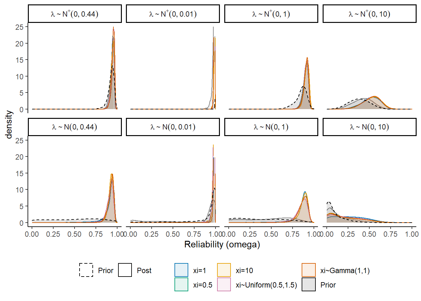
ggsave(filename = "fig/study4_posterior_sensitity_omega.pdf",plot=p,width = 7.66, height=4.5,units="in")
ggsave(filename = "fig/study4_posterior_sensitity_omega.png",plot=p,width = 7.66, height=4.5,units="in")


# numerically describe due to how close all posteriors were
f <- function(x){
  c(mean(x, na.rm=T), sd(x, na.rm=T), quantile(x, c(0.025, 0.25, 0.5, 0.75, 0.975), na.rm=T))
}

post.sum <- plot.post %>%
  group_by(Prior, xi) %>%
  summarise(
    Mean = mean(omega, na.rm=T),
    SD = sd(omega, na.rm=T),
    q025 = quantile(omega, c(0.025), na.rm=T),
    q25 = quantile(omega, c(0.25), na.rm=T),
    q50 = quantile(omega, c(0.5), na.rm=T),
    q75 = quantile(omega, c(0.75), na.rm=T),
    q975 = quantile(omega, c(0.975), na.rm=T)
  )
`summarise()` has grouped output by 'Prior'. You can override using the `.groups` argument.kable(post.sum, format="html", digits=3)%>%
kable_styling(full_width = T)| Prior | xi | Mean | SD | q025 | q25 | q50 | q75 | q975 |
|---|---|---|---|---|---|---|---|---|
| Alt_A.Alt_A | Alt_A | 0.974 | 0.019 | 0.924 | 0.969 | 0.980 | 0.987 | 0.991 |
| Alt_A.Alt_B | Alt_B | 0.987 | 0.005 | 0.973 | 0.986 | 0.988 | 0.990 | 0.993 |
| Alt_A.Alt_C | Alt_C | 0.987 | 0.005 | 0.975 | 0.984 | 0.989 | 0.992 | 0.994 |
| Alt_A.Alt_D | Alt_D | 0.987 | 0.006 | 0.972 | 0.983 | 0.988 | 0.991 | 0.994 |
| Alt_A.Base | Base | 0.988 | 0.005 | 0.976 | 0.985 | 0.989 | 0.991 | 0.993 |
| Alt_B.Alt_A | Alt_A | 0.901 | 0.031 | 0.826 | 0.886 | 0.907 | 0.923 | 0.945 |
| Alt_B.Alt_B | Alt_B | 0.914 | 0.028 | 0.848 | 0.898 | 0.918 | 0.934 | 0.955 |
| Alt_B.Alt_C | Alt_C | 0.908 | 0.030 | 0.835 | 0.893 | 0.912 | 0.928 | 0.949 |
| Alt_B.Alt_D | Alt_D | 0.908 | 0.028 | 0.838 | 0.893 | 0.914 | 0.929 | 0.948 |
| Alt_B.Base | Base | 0.903 | 0.030 | 0.833 | 0.885 | 0.908 | 0.924 | 0.948 |
| Alt_C.Alt_A | Alt_A | 0.420 | 0.113 | 0.196 | 0.345 | 0.427 | 0.500 | 0.626 |
| Alt_C.Alt_B | Alt_B | 0.524 | 0.104 | 0.300 | 0.457 | 0.534 | 0.599 | 0.702 |
| Alt_C.Alt_C | Alt_C | 0.525 | 0.097 | 0.320 | 0.462 | 0.533 | 0.596 | 0.693 |
| Alt_C.Alt_D | Alt_D | 0.524 | 0.100 | 0.309 | 0.460 | 0.535 | 0.596 | 0.694 |
| Alt_C.Base | Base | 0.514 | 0.103 | 0.293 | 0.448 | 0.522 | 0.591 | 0.686 |
| Alt_D.Alt_A | Alt_A | 0.921 | 0.043 | 0.804 | 0.906 | 0.932 | 0.949 | 0.967 |
| Alt_D.Alt_B | Alt_B | 0.920 | 0.032 | 0.838 | 0.906 | 0.926 | 0.942 | 0.962 |
| Alt_D.Alt_C | Alt_C | 0.911 | 0.047 | 0.797 | 0.893 | 0.923 | 0.940 | 0.964 |
| Alt_D.Alt_D | Alt_D | 0.924 | 0.033 | 0.845 | 0.907 | 0.932 | 0.948 | 0.966 |
| Alt_D.Base | Base | 0.908 | 0.069 | 0.699 | 0.894 | 0.931 | 0.948 | 0.965 |
| Alt_E.Alt_A | Alt_A | 0.790 | 0.331 | 0.008 | 0.819 | 0.971 | 0.979 | 0.986 |
| Alt_E.Alt_B | Alt_B | 0.977 | 0.014 | 0.941 | 0.972 | 0.981 | 0.986 | 0.991 |
| Alt_E.Alt_C | Alt_C | 0.976 | 0.019 | 0.929 | 0.972 | 0.981 | 0.986 | 0.992 |
| Alt_E.Alt_D | Alt_D | 0.983 | 0.007 | 0.964 | 0.981 | 0.985 | 0.988 | 0.993 |
| Alt_E.Base | Base | 0.982 | 0.012 | 0.946 | 0.980 | 0.986 | 0.990 | 0.994 |
| Alt_F.Alt_A | Alt_A | 0.449 | 0.268 | 0.003 | 0.211 | 0.492 | 0.687 | 0.840 |
| Alt_F.Alt_B | Alt_B | 0.874 | 0.057 | 0.724 | 0.852 | 0.887 | 0.914 | 0.942 |
| Alt_F.Alt_C | Alt_C | 0.855 | 0.069 | 0.667 | 0.824 | 0.870 | 0.904 | 0.938 |
| Alt_F.Alt_D | Alt_D | 0.870 | 0.059 | 0.731 | 0.841 | 0.882 | 0.911 | 0.944 |
| Alt_F.Base | Base | 0.863 | 0.079 | 0.623 | 0.847 | 0.884 | 0.908 | 0.943 |
| Alt_G.Alt_A | Alt_A | 0.122 | 0.128 | 0.000 | 0.019 | 0.075 | 0.189 | 0.449 |
| Alt_G.Alt_B | Alt_B | 0.187 | 0.166 | 0.000 | 0.039 | 0.140 | 0.310 | 0.544 |
| Alt_G.Alt_C | Alt_C | 0.211 | 0.172 | 0.001 | 0.052 | 0.180 | 0.341 | 0.570 |
| Alt_G.Alt_D | Alt_D | 0.195 | 0.175 | 0.000 | 0.036 | 0.151 | 0.322 | 0.578 |
| Alt_G.Base | Base | 0.254 | 0.178 | 0.001 | 0.099 | 0.243 | 0.393 | 0.601 |
| Base.Alt_A | Alt_A | 0.938 | 0.021 | 0.886 | 0.927 | 0.943 | 0.955 | 0.967 |
| Base.Alt_B | Alt_B | 0.943 | 0.020 | 0.894 | 0.933 | 0.947 | 0.959 | 0.971 |
| Base.Alt_C | Alt_C | 0.946 | 0.019 | 0.897 | 0.937 | 0.952 | 0.960 | 0.971 |
| Base.Alt_D | Alt_D | 0.950 | 0.020 | 0.898 | 0.942 | 0.955 | 0.964 | 0.977 |
| Base.Base | Base | 0.945 | 0.020 | 0.894 | 0.935 | 0.948 | 0.959 | 0.972 |
print(
  xtable(
    post.sum
    , caption = c("Summary of posterior distributions")
  ),
  include.rownames=F,
  booktabs=T
)
% latex table generated in R 4.0.5 by xtable 1.8-4 package
% Tue Feb 15 13:00:40 2022
\begin{table}[ht]
\centering
\begin{tabular}{llrrrrrrr}
\toprule
Prior & xi & Mean & SD & q025 & q25 & q50 & q75 & q975 \\
\midrule
Alt\_A.Alt\_A & Alt\_A & 0.97 & 0.02 & 0.92 & 0.97 & 0.98 & 0.99 & 0.99 \\
Alt\_A.Alt\_B & Alt\_B & 0.99 & 0.01 & 0.97 & 0.99 & 0.99 & 0.99 & 0.99 \\
Alt\_A.Alt\_C & Alt\_C & 0.99 & 0.01 & 0.97 & 0.98 & 0.99 & 0.99 & 0.99 \\
Alt\_A.Alt\_D & Alt\_D & 0.99 & 0.01 & 0.97 & 0.98 & 0.99 & 0.99 & 0.99 \\
Alt\_A.Base & Base & 0.99 & 0.00 & 0.98 & 0.98 & 0.99 & 0.99 & 0.99 \\
Alt\_B.Alt\_A & Alt\_A & 0.90 & 0.03 & 0.83 & 0.89 & 0.91 & 0.92 & 0.94 \\
Alt\_B.Alt\_B & Alt\_B & 0.91 & 0.03 & 0.85 & 0.90 & 0.92 & 0.93 & 0.96 \\
Alt\_B.Alt\_C & Alt\_C & 0.91 & 0.03 & 0.84 & 0.89 & 0.91 & 0.93 & 0.95 \\
Alt\_B.Alt\_D & Alt\_D & 0.91 & 0.03 & 0.84 & 0.89 & 0.91 & 0.93 & 0.95 \\
Alt\_B.Base & Base & 0.90 & 0.03 & 0.83 & 0.89 & 0.91 & 0.92 & 0.95 \\
Alt\_C.Alt\_A & Alt\_A & 0.42 & 0.11 & 0.20 & 0.34 & 0.43 & 0.50 & 0.63 \\
Alt\_C.Alt\_B & Alt\_B & 0.52 & 0.10 & 0.30 & 0.46 & 0.53 & 0.60 & 0.70 \\
Alt\_C.Alt\_C & Alt\_C & 0.53 & 0.10 & 0.32 & 0.46 & 0.53 & 0.60 & 0.69 \\
Alt\_C.Alt\_D & Alt\_D & 0.52 & 0.10 & 0.31 & 0.46 & 0.53 & 0.60 & 0.69 \\
Alt\_C.Base & Base & 0.51 & 0.10 & 0.29 & 0.45 & 0.52 & 0.59 & 0.69 \\
Alt\_D.Alt\_A & Alt\_A & 0.92 & 0.04 & 0.80 & 0.91 & 0.93 & 0.95 & 0.97 \\
Alt\_D.Alt\_B & Alt\_B & 0.92 & 0.03 & 0.84 & 0.91 & 0.93 & 0.94 & 0.96 \\
Alt\_D.Alt\_C & Alt\_C & 0.91 & 0.05 & 0.80 & 0.89 & 0.92 & 0.94 & 0.96 \\
Alt\_D.Alt\_D & Alt\_D & 0.92 & 0.03 & 0.84 & 0.91 & 0.93 & 0.95 & 0.97 \\
Alt\_D.Base & Base & 0.91 & 0.07 & 0.70 & 0.89 & 0.93 & 0.95 & 0.97 \\
Alt\_E.Alt\_A & Alt\_A & 0.79 & 0.33 & 0.01 & 0.82 & 0.97 & 0.98 & 0.99 \\
Alt\_E.Alt\_B & Alt\_B & 0.98 & 0.01 & 0.94 & 0.97 & 0.98 & 0.99 & 0.99 \\
Alt\_E.Alt\_C & Alt\_C & 0.98 & 0.02 & 0.93 & 0.97 & 0.98 & 0.99 & 0.99 \\
Alt\_E.Alt\_D & Alt\_D & 0.98 & 0.01 & 0.96 & 0.98 & 0.98 & 0.99 & 0.99 \\
Alt\_E.Base & Base & 0.98 & 0.01 & 0.95 & 0.98 & 0.99 & 0.99 & 0.99 \\
Alt\_F.Alt\_A & Alt\_A & 0.45 & 0.27 & 0.00 & 0.21 & 0.49 & 0.69 & 0.84 \\
Alt\_F.Alt\_B & Alt\_B & 0.87 & 0.06 & 0.72 & 0.85 & 0.89 & 0.91 & 0.94 \\
Alt\_F.Alt\_C & Alt\_C & 0.85 & 0.07 & 0.67 & 0.82 & 0.87 & 0.90 & 0.94 \\
Alt\_F.Alt\_D & Alt\_D & 0.87 & 0.06 & 0.73 & 0.84 & 0.88 & 0.91 & 0.94 \\
Alt\_F.Base & Base & 0.86 & 0.08 & 0.62 & 0.85 & 0.88 & 0.91 & 0.94 \\
Alt\_G.Alt\_A & Alt\_A & 0.12 & 0.13 & 0.00 & 0.02 & 0.08 & 0.19 & 0.45 \\
Alt\_G.Alt\_B & Alt\_B & 0.19 & 0.17 & 0.00 & 0.04 & 0.14 & 0.31 & 0.54 \\
Alt\_G.Alt\_C & Alt\_C & 0.21 & 0.17 & 0.00 & 0.05 & 0.18 & 0.34 & 0.57 \\
Alt\_G.Alt\_D & Alt\_D & 0.20 & 0.18 & 0.00 & 0.04 & 0.15 & 0.32 & 0.58 \\
Alt\_G.Base & Base & 0.25 & 0.18 & 0.00 & 0.10 & 0.24 & 0.39 & 0.60 \\
Base.Alt\_A & Alt\_A & 0.94 & 0.02 & 0.89 & 0.93 & 0.94 & 0.95 & 0.97 \\
Base.Alt\_B & Alt\_B & 0.94 & 0.02 & 0.89 & 0.93 & 0.95 & 0.96 & 0.97 \\
Base.Alt\_C & Alt\_C & 0.95 & 0.02 & 0.90 & 0.94 & 0.95 & 0.96 & 0.97 \\
Base.Alt\_D & Alt\_D & 0.95 & 0.02 & 0.90 & 0.94 & 0.95 & 0.96 & 0.98 \\
Base.Base & Base & 0.94 & 0.02 & 0.89 & 0.94 & 0.95 & 0.96 & 0.97 \\
\bottomrule
\end{tabular}
\caption{Summary of posterior distributions}
\end{table}
sessionInfo()R version 4.0.5 (2021-03-31)
Platform: x86_64-w64-mingw32/x64 (64-bit)
Running under: Windows 10 x64 (build 22000)
Matrix products: default
locale:
[1] LC_COLLATE=English_United States.1252
[2] LC_CTYPE=English_United States.1252
[3] LC_MONETARY=English_United States.1252
[4] LC_NUMERIC=C
[5] LC_TIME=English_United States.1252
attached base packages:
[1] stats graphics grDevices utils datasets methods base
other attached packages:
[1] car_3.0-10 carData_3.0-4 mvtnorm_1.1-1
[4] LaplacesDemon_16.1.4 runjags_2.2.0-2 lme4_1.1-26
[7] Matrix_1.3-2 sirt_3.9-4 R2jags_0.6-1
[10] rjags_4-12 eRm_1.0-2 diffIRT_1.5
[13] statmod_1.4.35 xtable_1.8-4 kableExtra_1.3.4
[16] lavaan_0.6-7 polycor_0.7-10 bayesplot_1.8.0
[19] ggmcmc_1.5.1.1 coda_0.19-4 data.table_1.14.0
[22] patchwork_1.1.1 forcats_0.5.1 stringr_1.4.0
[25] dplyr_1.0.5 purrr_0.3.4 readr_1.4.0
[28] tidyr_1.1.3 tibble_3.1.0 ggplot2_3.3.5
[31] tidyverse_1.3.0 workflowr_1.6.2
loaded via a namespace (and not attached):
[1] minqa_1.2.4 TAM_3.5-19 colorspace_2.0-0 rio_0.5.26
[5] ellipsis_0.3.1 ggridges_0.5.3 rprojroot_2.0.2 fs_1.5.0
[9] rstudioapi_0.13 farver_2.1.0 fansi_0.4.2 lubridate_1.7.10
[13] xml2_1.3.2 codetools_0.2-18 splines_4.0.5 mnormt_2.0.2
[17] knitr_1.31 jsonlite_1.7.2 nloptr_1.2.2.2 broom_0.7.5
[21] dbplyr_2.1.0 compiler_4.0.5 httr_1.4.2 backports_1.2.1
[25] assertthat_0.2.1 cli_2.3.1 later_1.1.0.1 htmltools_0.5.1.1
[29] tools_4.0.5 gtable_0.3.0 glue_1.4.2 Rcpp_1.0.7
[33] cellranger_1.1.0 jquerylib_0.1.3 vctrs_0.3.6 svglite_2.0.0
[37] nlme_3.1-152 psych_2.0.12 xfun_0.21 ps_1.6.0
[41] openxlsx_4.2.3 rvest_1.0.0 lifecycle_1.0.0 MASS_7.3-53.1
[45] scales_1.1.1 ragg_1.1.1 hms_1.0.0 promises_1.2.0.1
[49] parallel_4.0.5 RColorBrewer_1.1-2 curl_4.3 yaml_2.2.1
[53] sass_0.3.1 reshape_0.8.8 stringi_1.5.3 highr_0.8
[57] zip_2.1.1 boot_1.3-27 rlang_0.4.10 pkgconfig_2.0.3
[61] systemfonts_1.0.1 evaluate_0.14 lattice_0.20-41 labeling_0.4.2
[65] tidyselect_1.1.0 GGally_2.1.1 plyr_1.8.6 magrittr_2.0.1
[69] R6_2.5.0 generics_0.1.0 DBI_1.1.1 foreign_0.8-81
[73] pillar_1.5.1 haven_2.3.1 withr_2.4.1 abind_1.4-5
[77] modelr_0.1.8 crayon_1.4.1 utf8_1.1.4 tmvnsim_1.0-2
[81] rmarkdown_2.7 grid_4.0.5 readxl_1.3.1 CDM_7.5-15
[85] pbivnorm_0.6.0 git2r_0.28.0 reprex_1.0.0 digest_0.6.27
[89] webshot_0.5.2 httpuv_1.5.5 textshaping_0.3.1 stats4_4.0.5
[93] munsell_0.5.0 viridisLite_0.3.0 bslib_0.2.4 R2WinBUGS_2.1-21