Last updated: 2020-06-10

Checks: 6 1

Knit directory: mcfa-para-est/

This reproducible R Markdown analysis was created with workflowr (version 1.6.2). The Checks tab describes the reproducibility checks that were applied when the results were created. The Past versions tab lists the development history.

R Markdown file: uncommitted changes

The R Markdown is untracked by Git. To know which version of the R Markdown file created these results, you’ll want to first commit it to the Git repo. If you’re still working on the analysis, you can ignore this warning. When you’re finished, you can run wflow_publish to commit the R Markdown file and build the HTML.

Environment: empty

Great job! The global environment was empty. Objects defined in the global environment can affect the analysis in your R Markdown file in unknown ways. For reproduciblity it’s best to always run the code in an empty environment.

Seed: set.seed(20190614)

The command set.seed(20190614) was run prior to running the code in the R Markdown file. Setting a seed ensures that any results that rely on randomness, e.g. subsampling or permutations, are reproducible.

Session information: recorded

Great job! Recording the operating system, R version, and package versions is critical for reproducibility.

Cache: none

Nice! There were no cached chunks for this analysis, so you can be confident that you successfully produced the results during this run.

File paths: relative

Great job! Using relative paths to the files within your workflowr project makes it easier to run your code on other machines.

Repository version: eecb366

Great! You are using Git for version control. Tracking code development and connecting the code version to the results is critical for reproducibility.

The results in this page were generated with repository version eecb366. See the Past versions tab to see a history of the changes made to the R Markdown and HTML files.

Note that you need to be careful to ensure that all relevant files for the analysis have been committed to Git prior to generating the results (you can use wflow_publish or wflow_git_commit). workflowr only checks the R Markdown file, but you know if there are other scripts or data files that it depends on. Below is the status of the Git repository when the results were generated:


Ignored files:
    Ignored:    .Rhistory
    Ignored:    .Rproj.user/
    Ignored:    data/compiled_para_results.txt
    Ignored:    data/results_bias_est.csv
    Ignored:    data/results_bias_se.csv
    Ignored:    fig/
    Ignored:    manuscript/
    Ignored:    output/fact-cov-converge-largeN.pdf
    Ignored:    output/fact-cov-converge-medN.pdf
    Ignored:    output/fact-cov-converge-smallN.pdf
    Ignored:    output/loading-converge-largeN.pdf
    Ignored:    output/loading-converge-medN.pdf
    Ignored:    output/loading-converge-smallN.pdf
    Ignored:    references/
    Ignored:    sera-presentation/

Untracked files:
    Untracked:  analysis/ml-cfa-parameter-anova-estimates.Rmd
    Untracked:  analysis/ml-cfa-parameter-anova-relative-bias.Rmd
    Untracked:  analysis/ml-cfa-parameter-bias-latent-ICC.Rmd
    Untracked:  analysis/ml-cfa-parameter-bias-observed-ICC.Rmd
    Untracked:  analysis/ml-cfa-parameter-convergence-ARD-L1-factor-covariance.Rmd
    Untracked:  analysis/ml-cfa-parameter-convergence-ARD-L2-factor-covariance.Rmd
    Untracked:  analysis/ml-cfa-parameter-convergence-ARD-L2-factor-variance.Rmd
    Untracked:  analysis/ml-cfa-parameter-convergence-ARD-L2-residual-variance.Rmd
    Untracked:  analysis/ml-cfa-parameter-convergence-ARD-factor-loadings.Rmd
    Untracked:  analysis/ml-cfa-parameter-convergence-ARD-latent-ICC.Rmd
    Untracked:  analysis/ml-cfa-parameter-convergence-ARD-observed-ICC.Rmd
    Untracked:  analysis/ml-cfa-parameter-convergence-correlation-pubfigure.Rmd
    Untracked:  analysis/ml-cfa-parameter-convergence-trace-plots-factor-loadings.Rmd
    Untracked:  analysis/ml-cfa-standard-error-anova-logSE.Rmd
    Untracked:  analysis/ml-cfa-standard-error-anova-relative-bias.Rmd
    Untracked:  analysis/ml-cfa-standard-error-bias-factor-loadings.Rmd
    Untracked:  analysis/ml-cfa-standard-error-bias-level1-factor-covariances.Rmd
    Untracked:  analysis/ml-cfa-standard-error-bias-level2-factor-covariances.Rmd
    Untracked:  analysis/ml-cfa-standard-error-bias-level2-factor-variances.Rmd
    Untracked:  analysis/ml-cfa-standard-error-bias-level2-residual-variances.Rmd
    Untracked:  analysis/ml-cfa-standard-error-bias-overview.Rmd
    Untracked:  code/r_functions.R
    Untracked:  renv.lock
    Untracked:  renv/

Unstaged changes:
    Modified:   .gitignore
    Modified:   analysis/index.Rmd
    Modified:   analysis/ml-cfa-convergence-summary.Rmd
    Modified:   analysis/ml-cfa-parameter-bias-factor-loadings.Rmd
    Modified:   analysis/ml-cfa-parameter-bias-level1-factor-covariances.Rmd
    Modified:   analysis/ml-cfa-parameter-bias-level2-factor-covariances.Rmd
    Modified:   analysis/ml-cfa-parameter-bias-level2-factor-variances.Rmd
    Modified:   analysis/ml-cfa-parameter-bias-level2-residual-variances.Rmd
    Modified:   analysis/ml-cfa-parameter-convergence-correlation-factor-loadings.Rmd
    Modified:   code/get_data.R
    Modified:   code/load_packages.R

Note that any generated files, e.g. HTML, png, CSS, etc., are not included in this status report because it is ok for generated content to have uncommitted changes.

There are no past versions. Publish this analysis with wflow_publish() to start tracking its development.

The purpose of this page is to identify the impact of design factors on parameter estimates. This is done using analysis of variance (factorial) on the parameter estimates.

Packages and Set-Up

rm(list=ls())
source(paste0(getwd(),"/code/load_packages.R"))
source(paste0(getwd(),"/code/get_data.R"))
source(paste0(getwd(),"/code/r_functions.R"))

# general options
theme_set(theme_bw())
options(digits=3)

##Chunk iptions
knitr::opts_chunk$set(out.width="225%")

Data Management

pvec <- c(paste0('lambda1',1:6), paste0('lambda2',6:10), 'psiW12','psiB1', 'psiB2', 'psiB12', paste0('thetaB',1:10))

# take out non-converged/inadmissible cases
sim_results <- filter(sim_results, Converge==1, Admissible==1)

# Set conditions levels as categorical values
sim_results <- sim_results %>%
  mutate(N1 = factor(N1, c("5", "10", "30")),
         N2 = factor(N2, c("30", "50", "100", "200")),
         ICC_OV = factor(ICC_OV, c("0.1","0.3", "0.5")),
         ICC_LV = factor(ICC_LV, c("0.1", "0.5")))

# convert to long format
long_results <- sim_results[,c("Condition", "Replication", "N1", "N2", "ICC_OV", "ICC_LV", "Estimator", pvec)] %>%
  pivot_longer(
    cols = all_of(pvec),
    names_to = "Parameter",
    values_to = "Estimate"
  )

Now, we are only going to do ANOVA on the estimates.

# Object to Story Results
resultsList <- list()

ANOVA and effect sizes for distributional differences

For this simulation experiment, there were 5 factors systematically varied. Of these 5 factors, 4 were factors influencing the observed data and 1 were factors pertaining to estimation and model fitting. The factors were

Level-1 sample size (5, 10, 30)
Level-2 sample size (30, 50, 100, 200)
Observed indicator ICC (.1, .3, .5)
Latent variable ICC (.1, .5)
Model estimator (MLR, ULSMV, WLSMV)

For each parameter SE, an analysis of variance (ANOVA) was conducted in order to test how much influence each of these design factors.

General Linear Model investigated for estimated parameters was: \[ Y_{ijklmn} = \mu + \alpha_{j} + \beta_{k} + \gamma_{l} + \delta_m + \theta_n +\\ (\alpha\beta)_{jk} + (\alpha\gamma)_{jl}+ (\alpha\delta)_{jm} + (\alpha\theta)_{jn}+ \\ (\beta\gamma)_{kl}+ (\beta\delta)_{km} + (\beta\theta)_{kn}+ (\gamma\delta)_{lm} + + (\gamma\theta)_{ln} + (\delta\theta)_{mn} + \varepsilon_{ijklmn} \] where

\(\mu\) is the grand mean,
\(\alpha_{j}\) is the effect of Level-1 sample size,
\(\beta_{k}\) is the effect of Level-2 sample size,
\(\gamma_{l}\) is the effect of Observed indicator ICC,
\(\delta_m\) is the effect of Latent variable ICC,
\(\theta_n\) is the effect of Model estimator ,
\((\alpha\beta)_{jk}\) is the interaction between Level-1 sample size and Level-2 sample size,
\((\alpha\gamma)_{jl}\) is the interaction between Level-1 sample size and Observed indicator ICC,
\((\alpha\delta)_{jm}\) is the interaction between Level-1 sample size and Latent variable ICC,
\((\alpha\theta)_{jn}\) is the interaction between Level-1 sample size and Model estimator ,
\((\beta\gamma)_{kl}\) is the interaction between Level-2 sample size and Observed indicator ICC,
\((\beta\delta)_{km}\) is the interaction between Level-2 sample size and Latent variable ICC,
\((\beta\theta)_{kn}\) is the interaction between Level-2 sample size and Model estimator ,
\((\gamma\delta)_{lm}\) is the interaction between Observed indicator ICC and Latent variable ICC,
\((\gamma\theta)_{ln}\) is the interaction between Observed indicator ICC and Model estimator ,
\((\delta\theta)_{mn}\) is the interaction between Latent variable ICC and Model estimator , and
\(\varepsilon_{ijklmn}\) is the residual error for the \(i^{th}\) observed SE estimate.

Note that for most of these terms there are actually 2 or 3 terms actually estimated. These additional terms are because of the categorical nature of each effect so we have to create “reference” groups and calculate the effect of being in a group other than the reference group. Higher order interactions were omitted for clarity of interpretation of the model. If interested in higher-order interactions, please see Maxwell and Delaney (2004).

The real reason the higher order interaction was omitted: Because I have no clue how to interpret a 5-way interaction (whatever the heck that is), I am limiting the ANOVA to all bivariate interactions.

Diagnostics for factorial ANOVA:

Independence of Observations
Normality of residuals across cells for the design
Homogeneity of variance across cells

Independence of observations is by design, where these data were randomly generated from a known population and observations are across replications and are independent. The normality assumptions is that the residuals of the models are normally distributed across the design cells. The normality assumption is tested by investigation by Shapiro-Wilks Test, the K-S test, and visual inspection of QQ-plots and histograms. The equality of variance is checked through Levene’s test across all the different conditions/groupings. Furthermore, the plots of the residuals are also indicative of the equality of variance across groups as there should be no apparent pattern to the residual plots.

Factor Loadings

Assumption Checking

sdat <- filter(long_results, Parameter %like% "lambda")

sdat <- sdat %>%
  group_by(Replication, N1, N2, ICC_OV, ICC_LV, Estimator) %>%
  summarise(Estimate = mean(Estimate))

# first, look at summary of Estimate Estimates
boxplot(sdat$Estimate)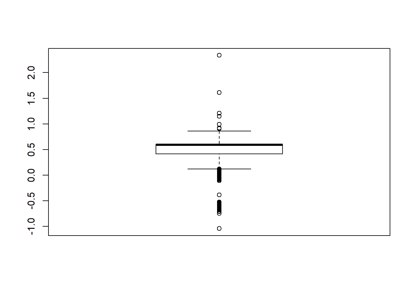

## model factors...
flist <- c('N1', 'N2', 'ICC_OV', 'ICC_LV', 'Estimator')
## Check assumptions
anova_assumptions_check(
  sdat, 'Estimate', factors = flist,
  model = as.formula('Estimate ~ N1 + N2 + ICC_OV + ICC_LV + Estimator + N1:N2 + N1:ICC_OV + N1:ICC_LV + N1:Estimator + N2:ICC_OV + N2:ICC_LV + N2:Estimator + ICC_OV:ICC_LV +  ICC_OV:Estimator  + ICC_LV:Estimator'))


 ============================= 

 Tests and Plots of Normality: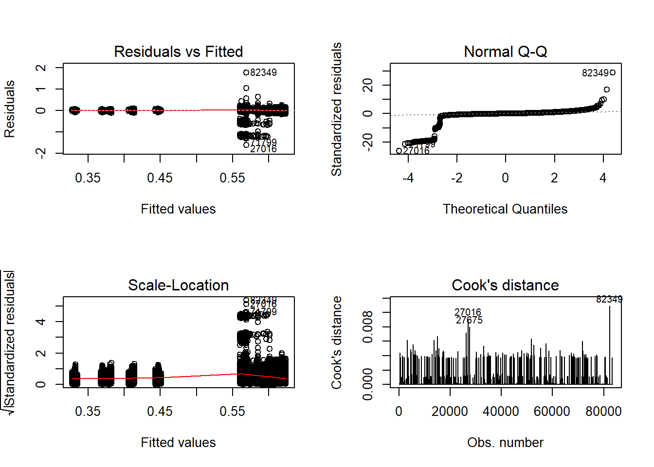


 Shapiro-Wilks Test of Normality of Residuals:

    Shapiro-Wilk normality test

data:  res
W = 0.3, p-value <2e-16


 K-S Test for Normality of Residuals:

    One-sample Kolmogorov-Smirnov test

data:  aov.out$residuals
D = 0.5, p-value <2e-16
alternative hypothesis: two-sided

`stat_bin()` using `bins = 30`. Pick better value with `binwidth`.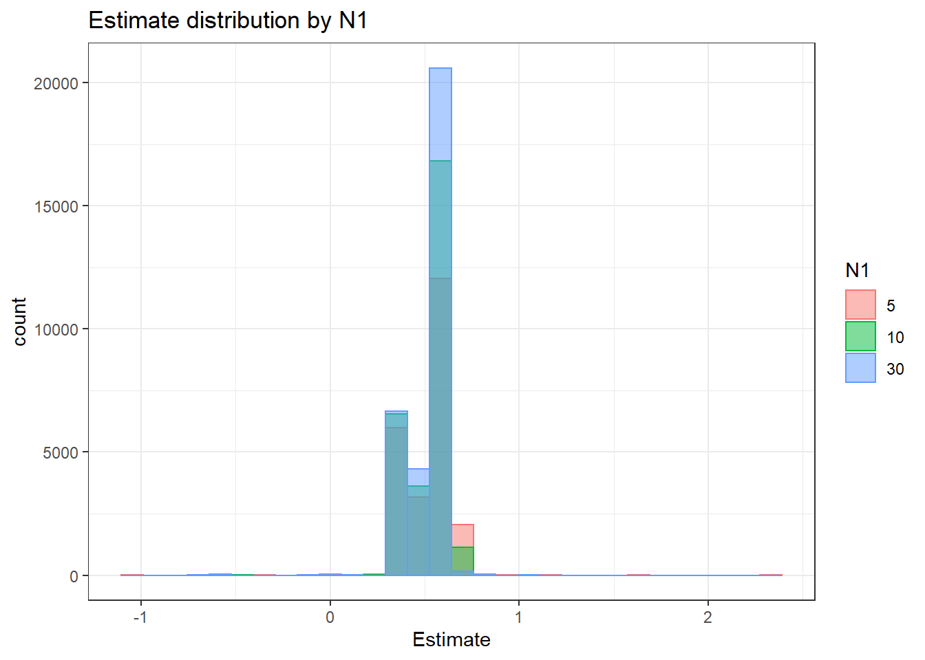

`stat_bin()` using `bins = 30`. Pick better value with `binwidth`.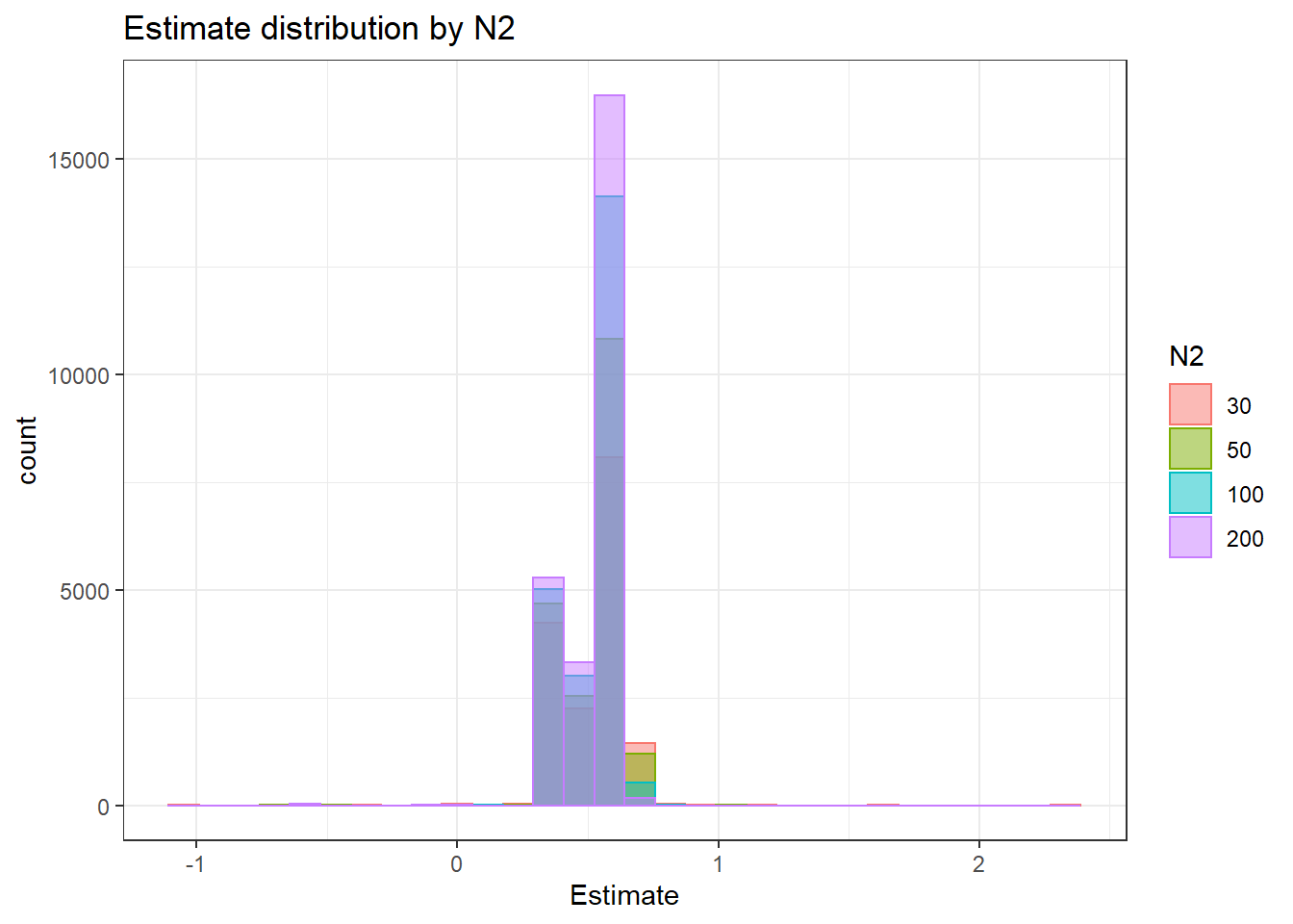

`stat_bin()` using `bins = 30`. Pick better value with `binwidth`.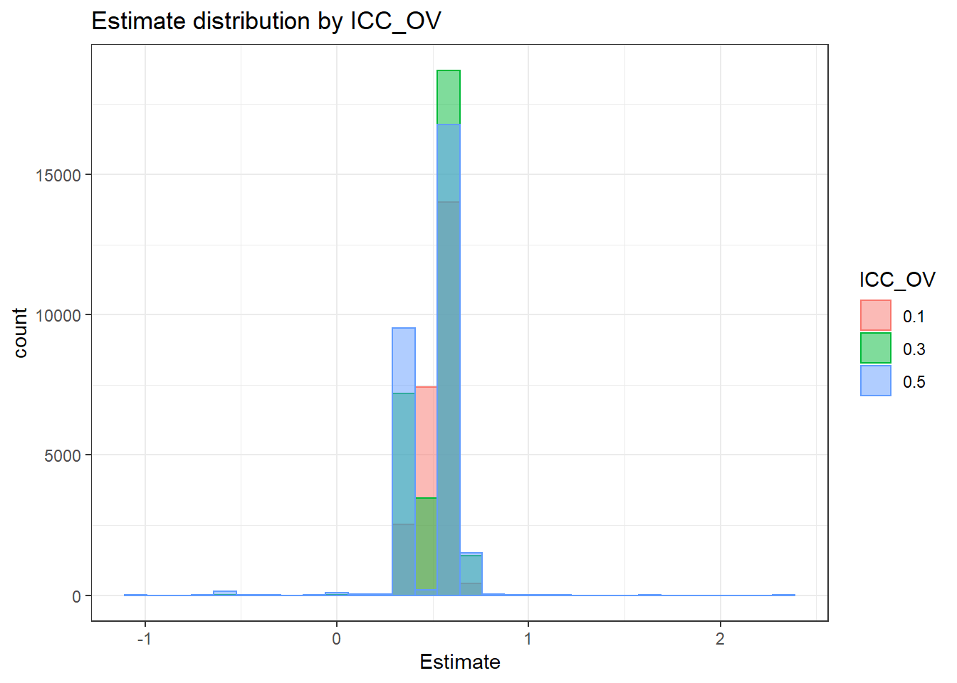

`stat_bin()` using `bins = 30`. Pick better value with `binwidth`.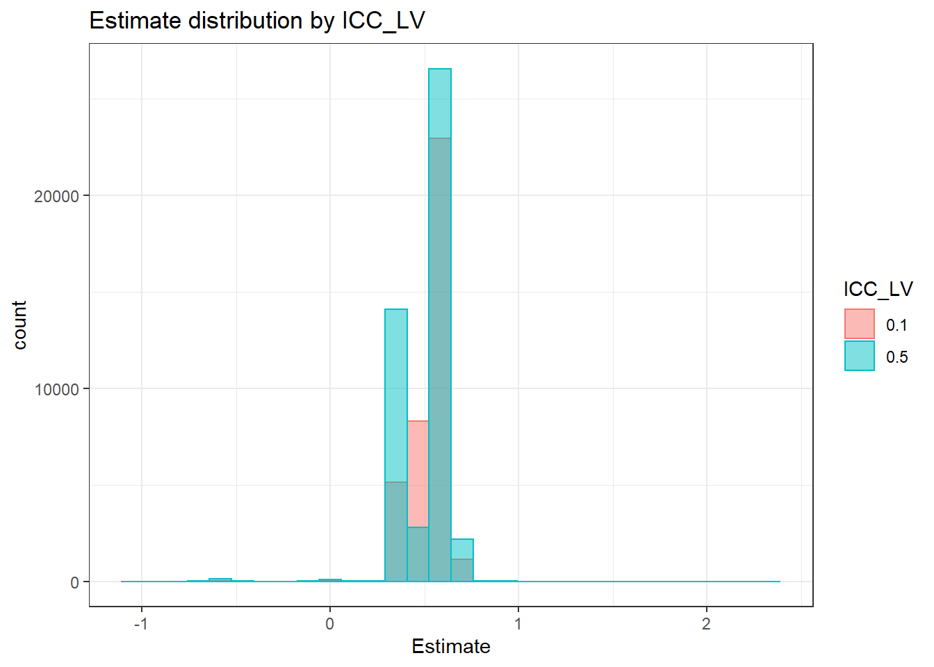

`stat_bin()` using `bins = 30`. Pick better value with `binwidth`.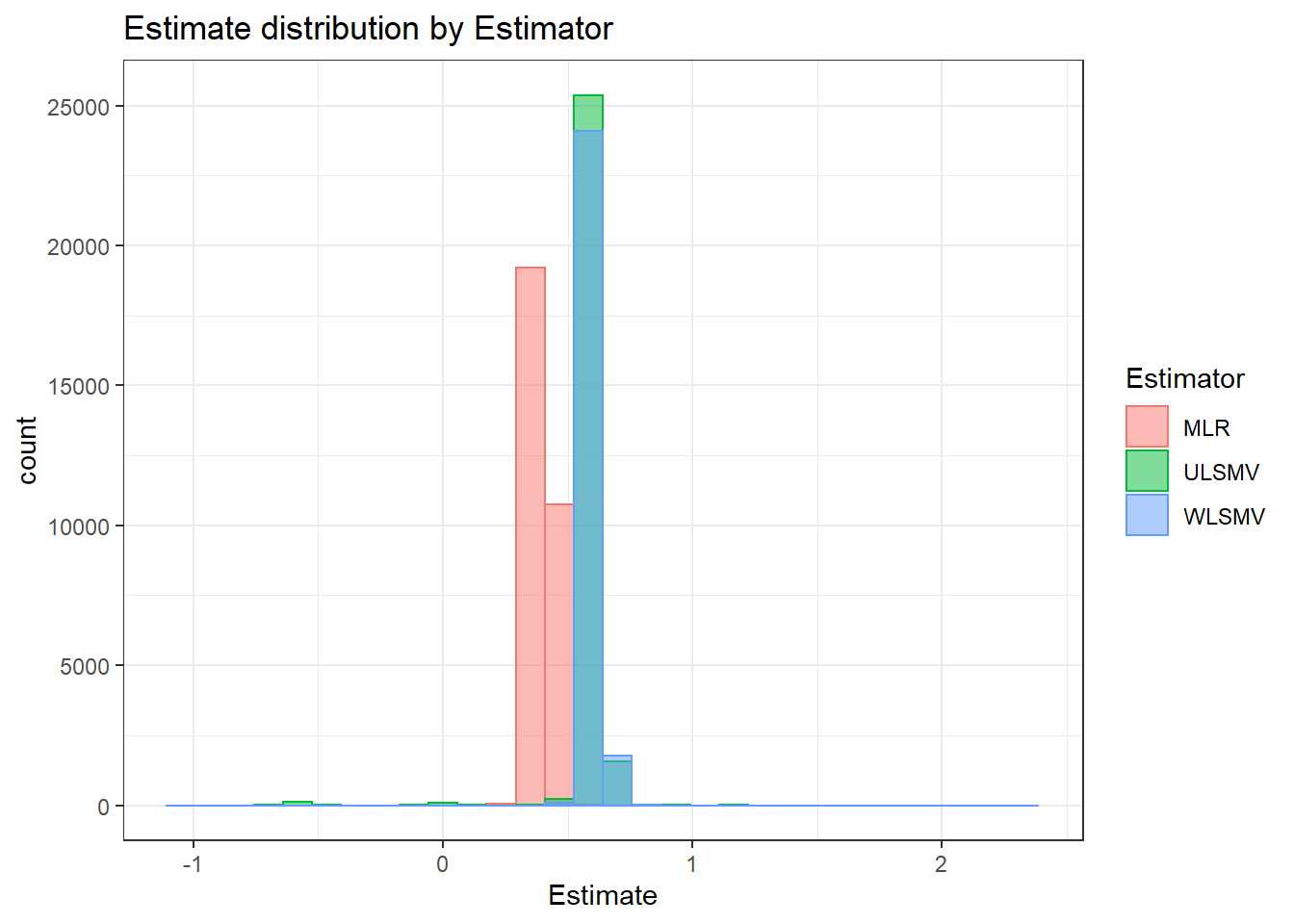


 ============================= 

 Tests of Homogeneity of Variance

 
 Levenes Test:  N1 
 
 
Levene's Test for Homogeneity of Variance (center = "mean")
         Df F value Pr(>F)    
group     2     206 <2e-16 ***
      83507                   
---
Signif. codes:  0 '***' 0.001 '**' 0.01 '*' 0.05 '.' 0.1 ' ' 1

 
 Levenes Test:  N2 
 
 
Levene's Test for Homogeneity of Variance (center = "mean")
         Df F value Pr(>F)    
group     3     216 <2e-16 ***
      83506                   
---
Signif. codes:  0 '***' 0.001 '**' 0.01 '*' 0.05 '.' 0.1 ' ' 1

 
 Levenes Test:  ICC_OV 
 
 
Levene's Test for Homogeneity of Variance (center = "mean")
         Df F value Pr(>F)    
group     2    3722 <2e-16 ***
      83507                   
---
Signif. codes:  0 '***' 0.001 '**' 0.01 '*' 0.05 '.' 0.1 ' ' 1

 
 Levenes Test:  ICC_LV 
 
 
Levene's Test for Homogeneity of Variance (center = "mean")
         Df F value Pr(>F)    
group     1    3934 <2e-16 ***
      83508                   
---
Signif. codes:  0 '***' 0.001 '**' 0.01 '*' 0.05 '.' 0.1 ' ' 1

 
 Levenes Test:  Estimator 
 
 
Levene's Test for Homogeneity of Variance (center = "mean")
         Df F value Pr(>F)    
group     2     560 <2e-16 ***
      83507                   
---
Signif. codes:  0 '***' 0.001 '**' 0.01 '*' 0.05 '.' 0.1 ' ' 1

ANOVA Results

model = as.formula('Estimate ~ N1 + N2 + ICC_OV + ICC_LV + Estimator + N1:N2 + N1:ICC_OV + N1:ICC_LV + N1:Estimator + N2:ICC_OV + N2:ICC_LV + N2:Estimator + ICC_OV:ICC_LV +  ICC_OV:Estimator  + ICC_LV:Estimator')

fit <- aov(model, data = sdat)
fit.out <- summary(fit)
fit.out

                    Df Sum Sq Mean Sq  F value  Pr(>F)    
N1                   2      1       0 8.61e+01 < 2e-16 ***
N2                   3      2       1 1.75e+02 < 2e-16 ***
ICC_OV               2     10       5 1.30e+03 < 2e-16 ***
ICC_LV               1      7       7 1.78e+03 < 2e-16 ***
Estimator            2    837     419 1.11e+05 < 2e-16 ***
N1:N2                6      0       0 5.28e+00 1.9e-05 ***
N1:ICC_OV            4      0       0 1.57e+00    0.18    
N1:ICC_LV            2      0       0 1.14e+00    0.32    
N1:Estimator         4      1       0 4.83e+01 < 2e-16 ***
N2:ICC_OV            6      0       0 1.30e+01 9.9e-15 ***
N2:ICC_LV            3      0       0 1.39e+00    0.24    
N2:Estimator         6      1       0 4.23e+01 < 2e-16 ***
ICC_OV:ICC_LV        2      0       0 3.21e+01 1.2e-14 ***
ICC_OV:Estimator     4     18       4 1.17e+03 < 2e-16 ***
ICC_LV:Estimator     2      5       2 6.09e+02 < 2e-16 ***
Residuals        83460    315       0                     
---
Signif. codes:  0 '***' 0.001 '**' 0.01 '*' 0.05 '.' 0.1 ' ' 1

resultsList[["FactorLoadings"]] <- cbind(omega2(fit.out), p_omega2(fit.out))
resultsList[["FactorLoadings"]]

                 omega^2 partial-omega^2
N1                0.0005          0.0020
N2                0.0016          0.0062
ICC_OV            0.0082          0.0303
ICC_LV            0.0056          0.0209
Estimator         0.6997          0.7263
N1:N2             0.0001          0.0003
N1:ICC_OV         0.0000          0.0000
N1:ICC_LV         0.0000          0.0000
N1:Estimator      0.0006          0.0023
N2:ICC_OV         0.0002          0.0009
N2:ICC_LV         0.0000          0.0000
N2:Estimator      0.0008          0.0030
ICC_OV:ICC_LV     0.0002          0.0007
ICC_OV:Estimator  0.0148          0.0532
ICC_LV:Estimator  0.0038          0.0144

Level-1 factor Covariance

Assumption Checking

sdat <- filter(long_results, Parameter %like% "psiW")

sdat <- sdat %>%
  group_by(Replication, N1, N2, ICC_OV, ICC_LV, Estimator) %>%
  summarise(Estimate = mean(Estimate))

# first, look at summary of Estimate Estimates
boxplot(sdat$Estimate)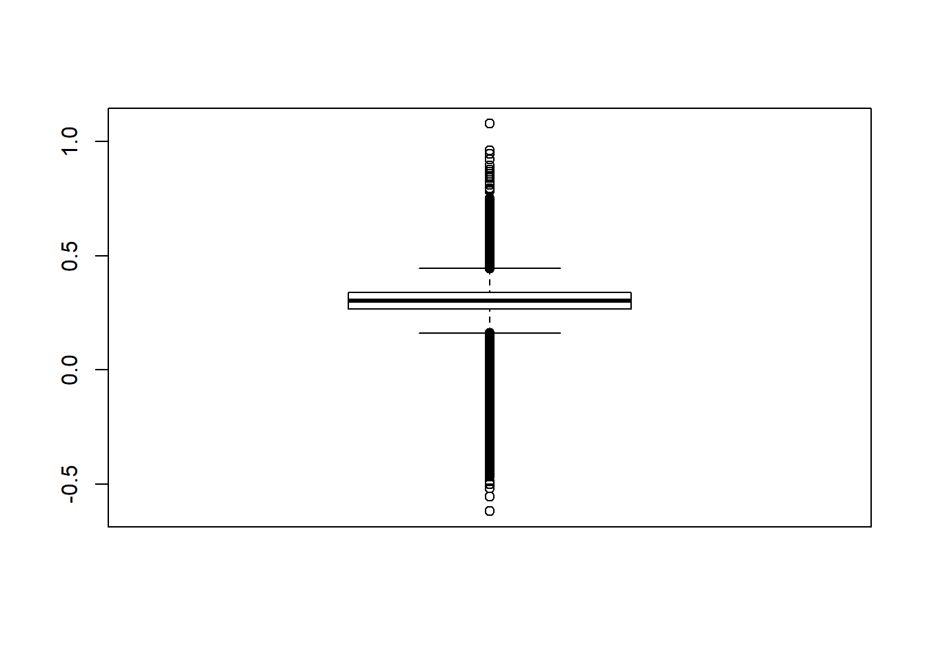

## model factors...
flist <- c('N1', 'N2', 'ICC_OV', 'ICC_LV', 'Estimator')
## Check assumptions
anova_assumptions_check(
  sdat, 'Estimate', factors = flist,
  model = as.formula('Estimate ~ N1 + N2 + ICC_OV + ICC_LV + Estimator + N1:N2 + N1:ICC_OV + N1:ICC_LV + N1:Estimator + N2:ICC_OV + N2:ICC_LV + N2:Estimator + ICC_OV:ICC_LV +  ICC_OV:Estimator  + ICC_LV:Estimator'))


 ============================= 

 Tests and Plots of Normality: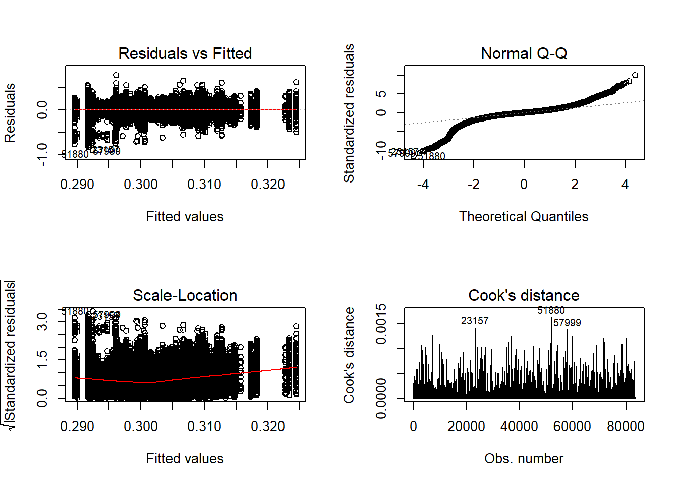


 Shapiro-Wilks Test of Normality of Residuals:

    Shapiro-Wilk normality test

data:  res
W = 0.9, p-value <2e-16


 K-S Test for Normality of Residuals:

    One-sample Kolmogorov-Smirnov test

data:  aov.out$residuals
D = 0.4, p-value <2e-16
alternative hypothesis: two-sided

`stat_bin()` using `bins = 30`. Pick better value with `binwidth`.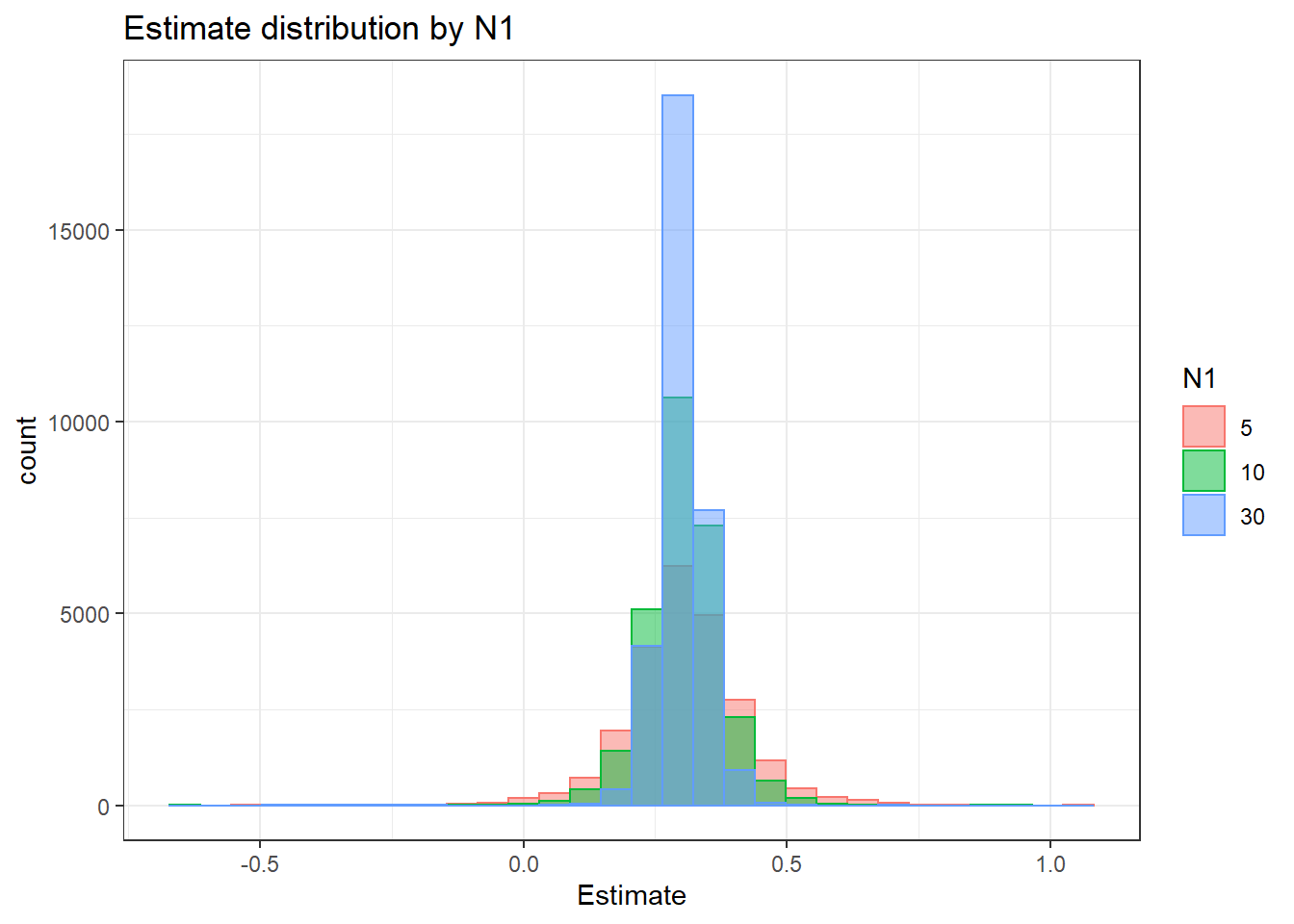

`stat_bin()` using `bins = 30`. Pick better value with `binwidth`.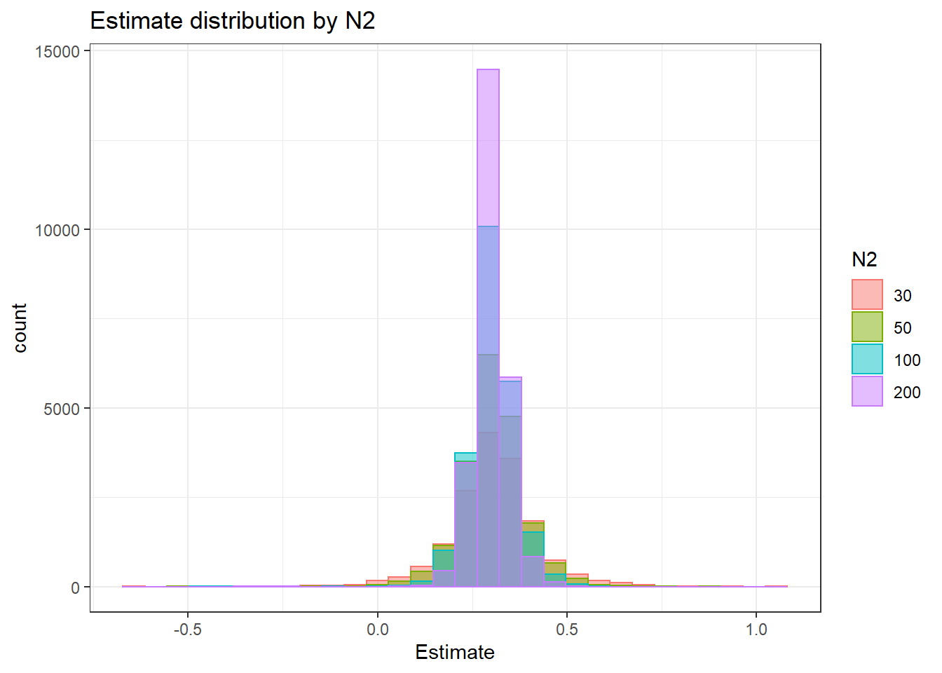

`stat_bin()` using `bins = 30`. Pick better value with `binwidth`.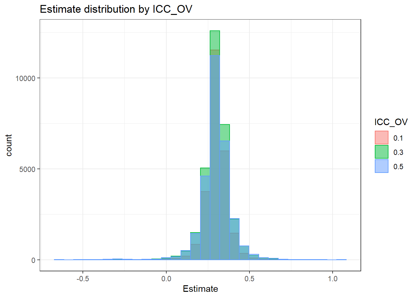

`stat_bin()` using `bins = 30`. Pick better value with `binwidth`.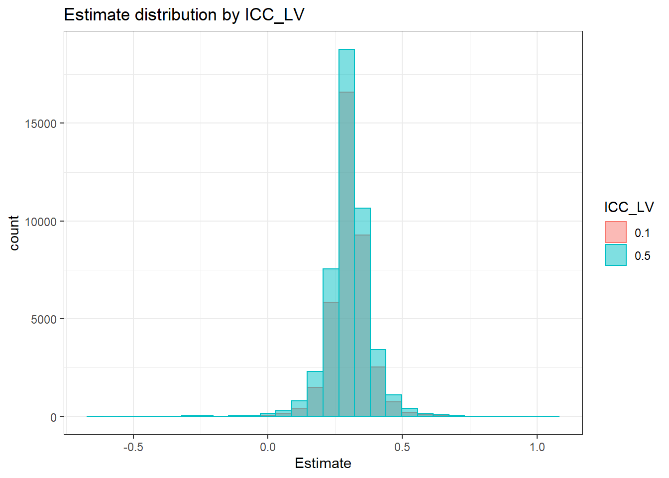

`stat_bin()` using `bins = 30`. Pick better value with `binwidth`.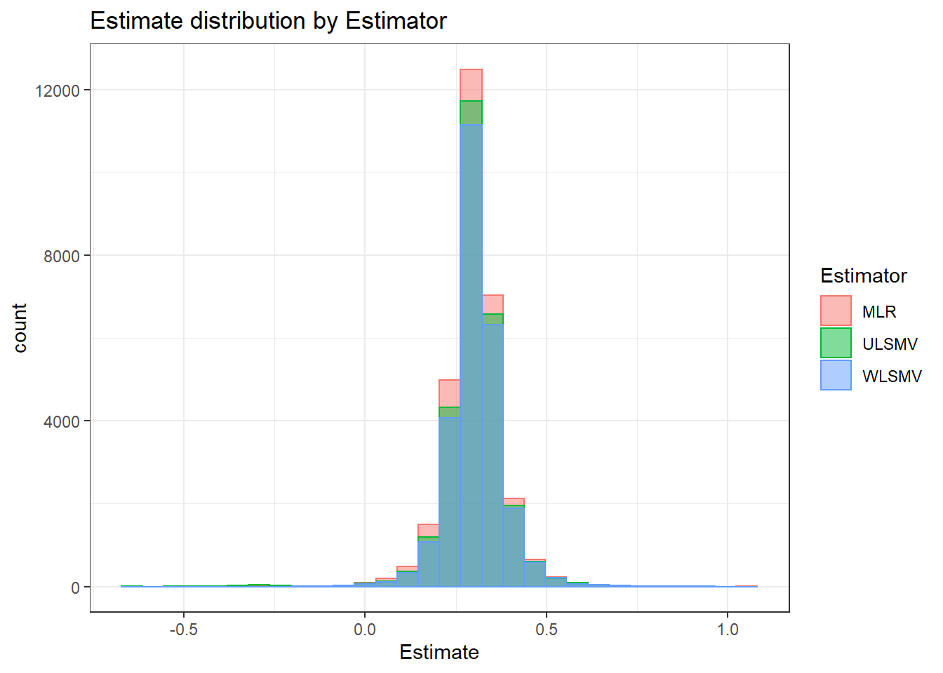


 ============================= 

 Tests of Homogeneity of Variance

 
 Levenes Test:  N1 
 
 
Levene's Test for Homogeneity of Variance (center = "mean")
         Df F value Pr(>F)    
group     2    5540 <2e-16 ***
      83507                   
---
Signif. codes:  0 '***' 0.001 '**' 0.01 '*' 0.05 '.' 0.1 ' ' 1

 
 Levenes Test:  N2 
 
 
Levene's Test for Homogeneity of Variance (center = "mean")
         Df F value Pr(>F)    
group     3    3105 <2e-16 ***
      83506                   
---
Signif. codes:  0 '***' 0.001 '**' 0.01 '*' 0.05 '.' 0.1 ' ' 1

 
 Levenes Test:  ICC_OV 
 
 
Levene's Test for Homogeneity of Variance (center = "mean")
         Df F value Pr(>F)    
group     2     492 <2e-16 ***
      83507                   
---
Signif. codes:  0 '***' 0.001 '**' 0.01 '*' 0.05 '.' 0.1 ' ' 1

 
 Levenes Test:  ICC_LV 
 
 
Levene's Test for Homogeneity of Variance (center = "mean")
         Df F value Pr(>F)    
group     1     353 <2e-16 ***
      83508                   
---
Signif. codes:  0 '***' 0.001 '**' 0.01 '*' 0.05 '.' 0.1 ' ' 1

 
 Levenes Test:  Estimator 
 
 
Levene's Test for Homogeneity of Variance (center = "mean")
         Df F value  Pr(>F)    
group     2    26.4 3.3e-12 ***
      83507                    
---
Signif. codes:  0 '***' 0.001 '**' 0.01 '*' 0.05 '.' 0.1 ' ' 1

ANOVA Results

model = as.formula('Estimate ~ N1 + N2 + ICC_OV + ICC_LV + Estimator + N1:N2 + N1:ICC_OV + N1:ICC_LV + N1:Estimator + N2:ICC_OV + N2:ICC_LV + N2:Estimator + ICC_OV:ICC_LV +  ICC_OV:Estimator  + ICC_LV:Estimator')

fit <- aov(model, data = sdat)
fit.out <- summary(fit)
fit.out

                    Df Sum Sq Mean Sq F value  Pr(>F)    
N1                   2      0   0.040    6.53 0.00146 ** 
N2                   3      0   0.029    4.77 0.00250 ** 
ICC_OV               2      0   0.033    5.37 0.00468 ** 
ICC_LV               1      0   0.390   63.60 1.5e-15 ***
Estimator            2      0   0.146   23.88 4.3e-11 ***
N1:N2                6      0   0.003    0.47 0.82865    
N1:ICC_OV            4      0   0.019    3.05 0.01581 *  
N1:ICC_LV            2      0   0.145   23.68 5.2e-11 ***
N1:Estimator         4      0   0.022    3.54 0.00676 ** 
N2:ICC_OV            6      0   0.002    0.32 0.92465    
N2:ICC_LV            3      0   0.024    3.97 0.00768 ** 
N2:Estimator         6      0   0.025    4.08 0.00042 ***
ICC_OV:ICC_LV        2      0   0.022    3.64 0.02635 *  
ICC_OV:Estimator     4      0   0.038    6.13 6.2e-05 ***
ICC_LV:Estimator     2      0   0.109   17.81 1.9e-08 ***
Residuals        83460    511   0.006                    
---
Signif. codes:  0 '***' 0.001 '**' 0.01 '*' 0.05 '.' 0.1 ' ' 1

resultsList[["Level1-FactorCovariance"]] <- cbind(omega2(fit.out), p_omega2(fit.out))
resultsList[["Level1-FactorCovariance"]]

                 omega^2 partial-omega^2
N1                 1e-04           1e-04
N2                 1e-04           1e-04
ICC_OV             1e-04           1e-04
ICC_LV             7e-04           7e-04
Estimator          5e-04           5e-04
N1:N2              0e+00           0e+00
N1:ICC_OV          1e-04           1e-04
N1:ICC_LV          5e-04           5e-04
N1:Estimator       1e-04           1e-04
N2:ICC_OV          0e+00           0e+00
N2:ICC_LV          1e-04           1e-04
N2:Estimator       2e-04           2e-04
ICC_OV:ICC_LV      1e-04           1e-04
ICC_OV:Estimator   2e-04           2e-04
ICC_LV:Estimator   4e-04           4e-04

Level-2 factor (co)variances

Assumption Checking

sdat <- filter(long_results, Parameter %like% "psiB")

sdat <- sdat %>%
  group_by(Replication, N1, N2, ICC_OV, ICC_LV, Estimator) %>%
  summarise(Estimate = mean(Estimate))

# first, look at summary of Estimate Estimates
boxplot(sdat$Estimate)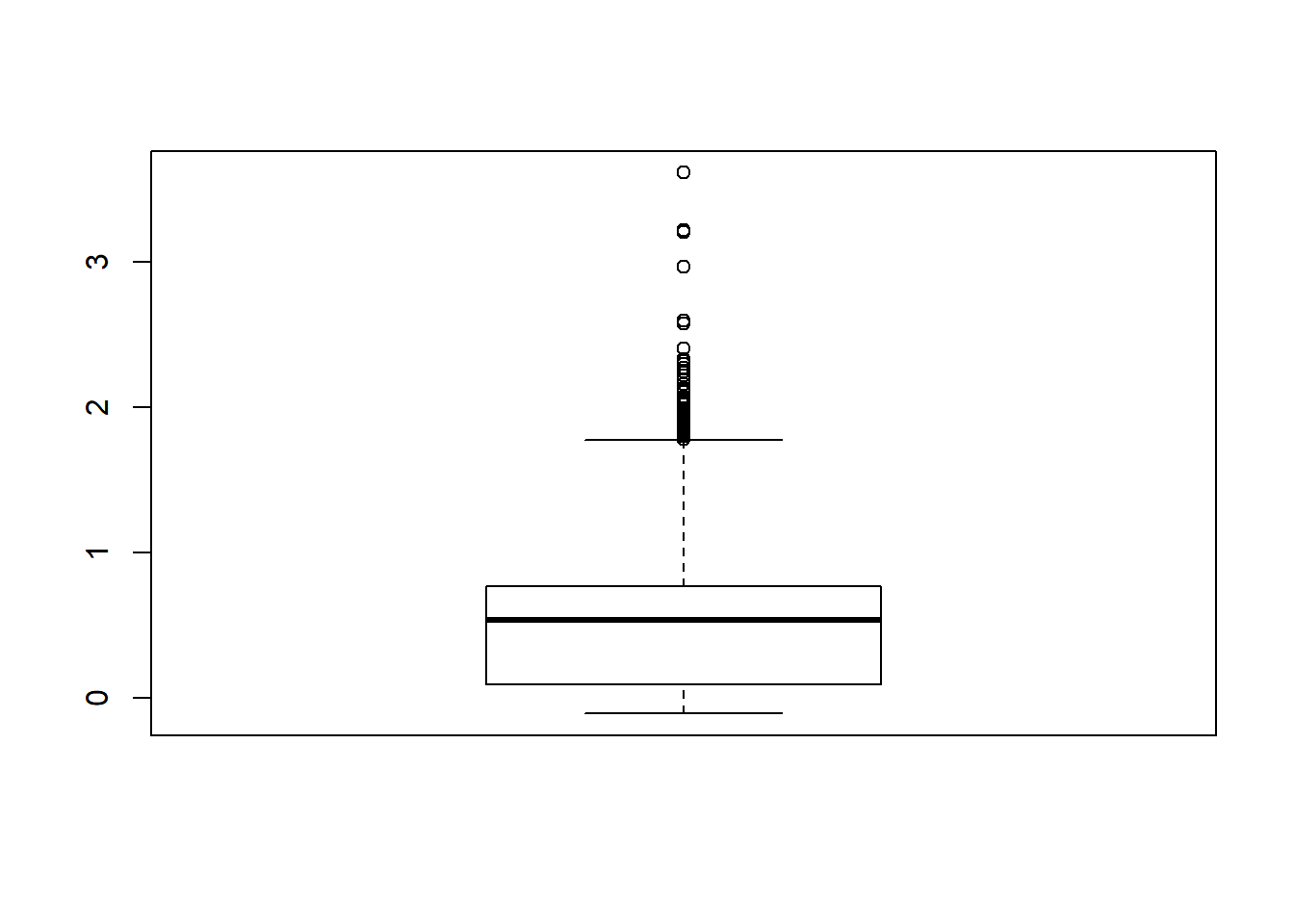

## model factors...
flist <- c('N1', 'N2', 'ICC_OV', 'ICC_LV', 'Estimator')
## Check assumptions
anova_assumptions_check(
  sdat, 'Estimate', factors = flist,
  model = as.formula('Estimate ~ N1 + N2 + ICC_OV + ICC_LV + Estimator + N1:N2 + N1:ICC_OV + N1:ICC_LV + N1:Estimator + N2:ICC_OV + N2:ICC_LV + N2:Estimator + ICC_OV:ICC_LV +  ICC_OV:Estimator  + ICC_LV:Estimator'))


 ============================= 

 Tests and Plots of Normality:


 Shapiro-Wilks Test of Normality of Residuals:

    Shapiro-Wilk normality test

data:  res
W = 0.9, p-value <2e-16


 K-S Test for Normality of Residuals:

Warning in ks.test(aov.out$residuals, "pnorm", alternative = "two.sided"): ties
should not be present for the Kolmogorov-Smirnov test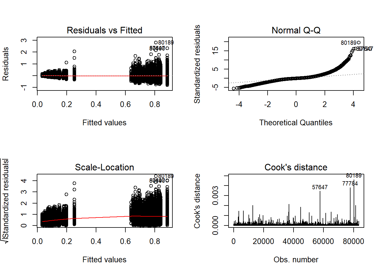


    One-sample Kolmogorov-Smirnov test

data:  aov.out$residuals
D = 0.4, p-value <2e-16
alternative hypothesis: two-sided

`stat_bin()` using `bins = 30`. Pick better value with `binwidth`.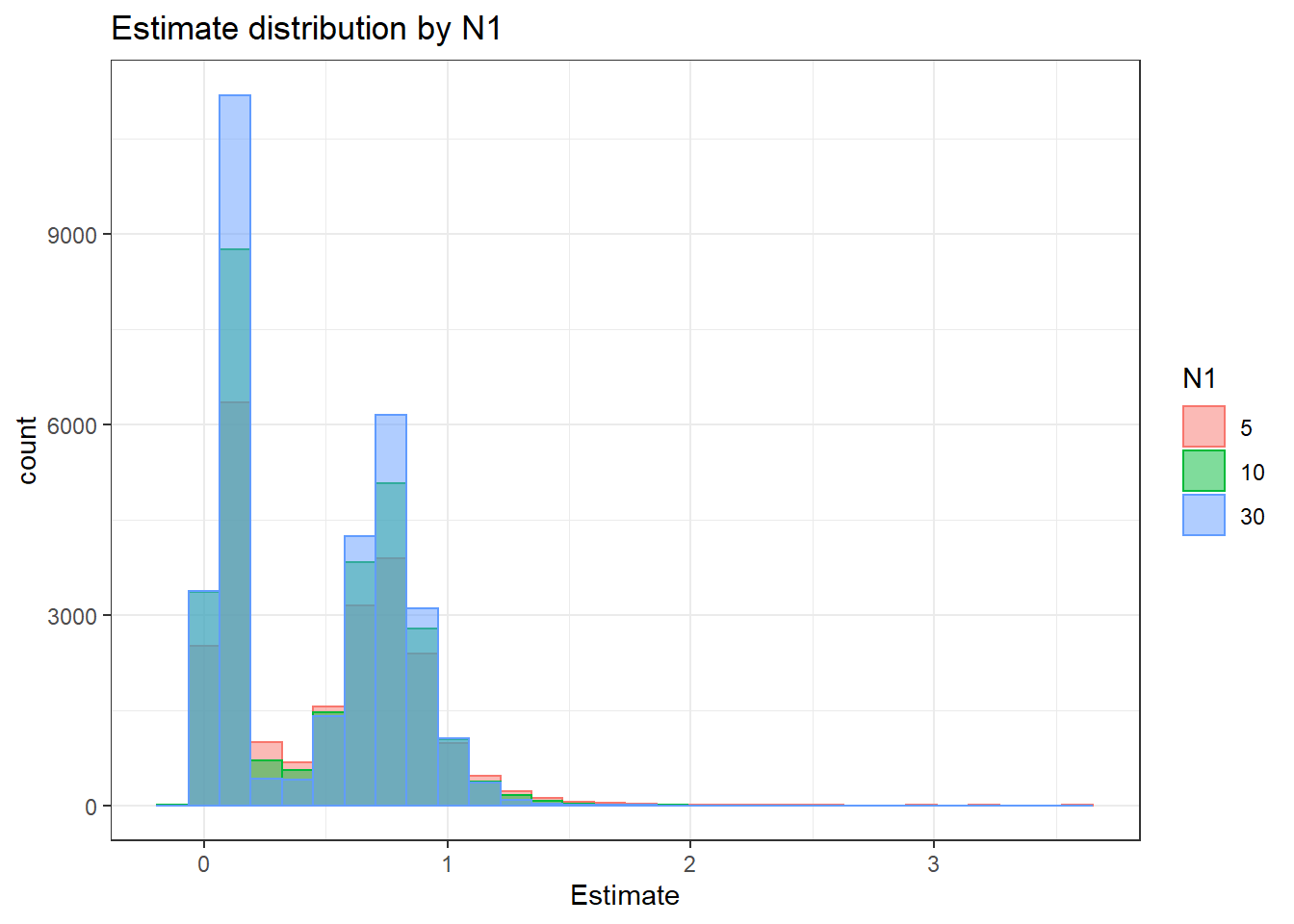

`stat_bin()` using `bins = 30`. Pick better value with `binwidth`.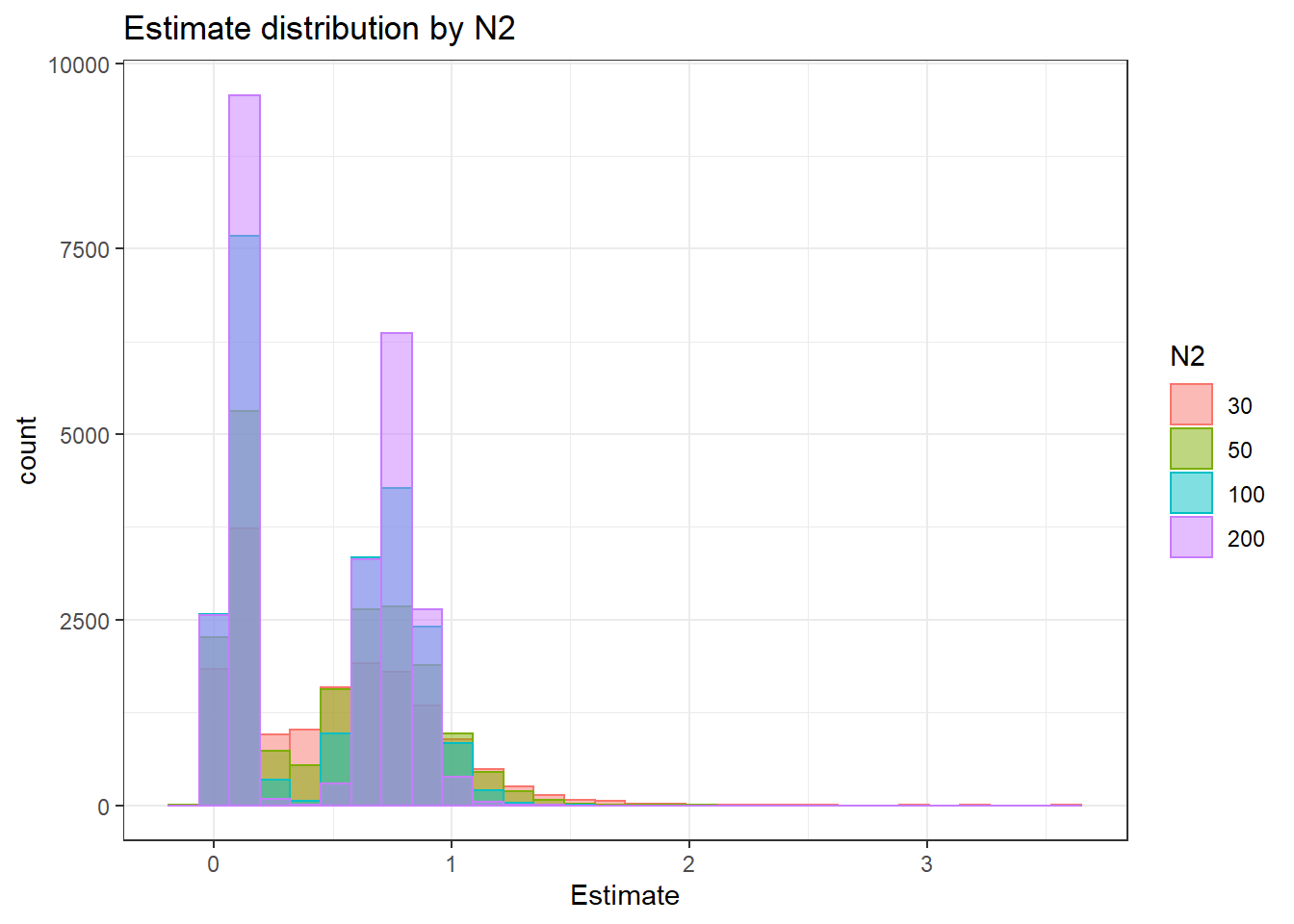

`stat_bin()` using `bins = 30`. Pick better value with `binwidth`.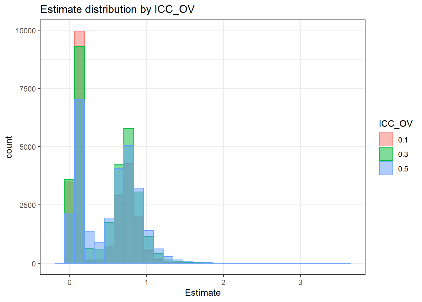

`stat_bin()` using `bins = 30`. Pick better value with `binwidth`.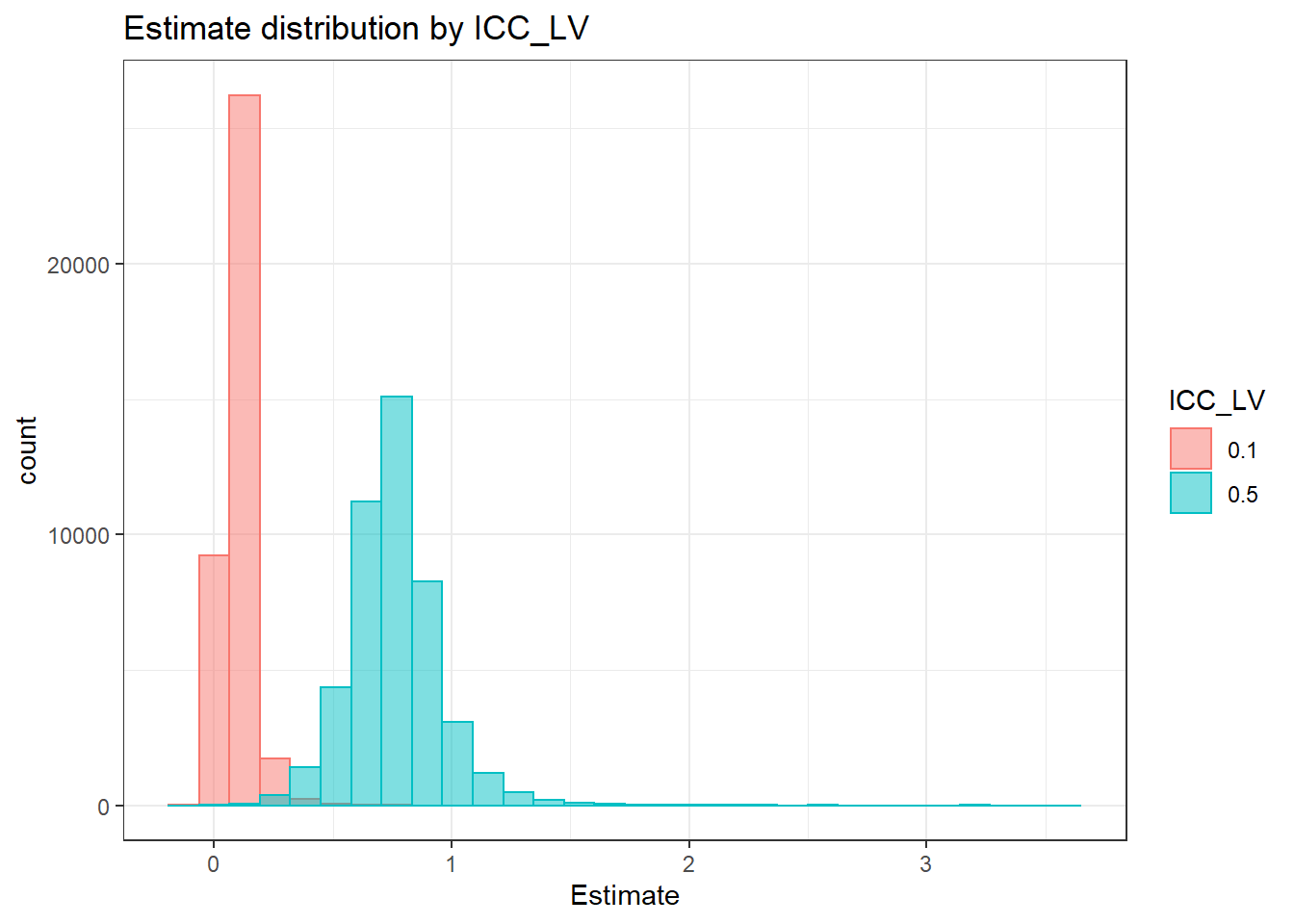

`stat_bin()` using `bins = 30`. Pick better value with `binwidth`.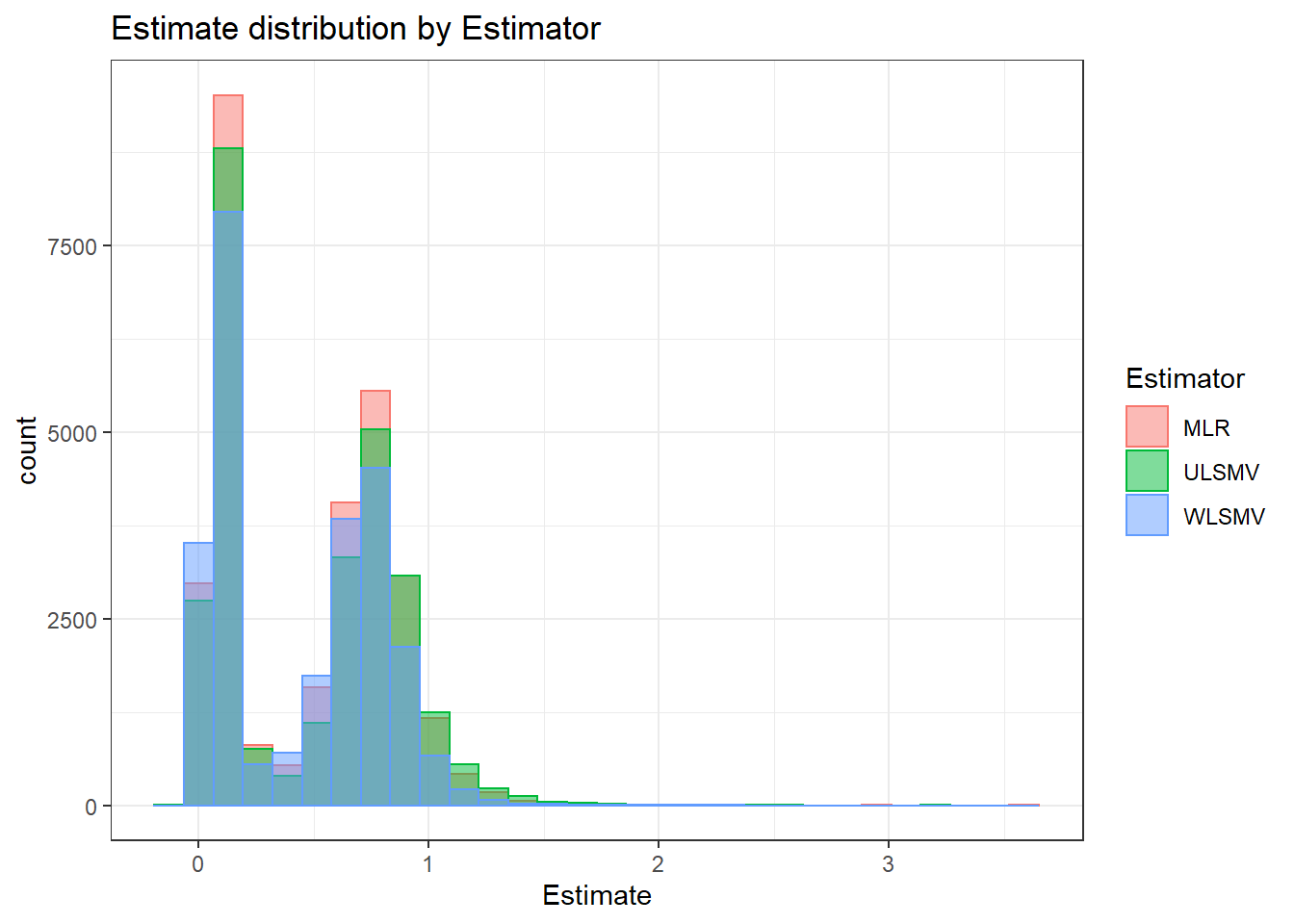


 ============================= 

 Tests of Homogeneity of Variance

 
 Levenes Test:  N1 
 
 
Levene's Test for Homogeneity of Variance (center = "mean")
         Df F value Pr(>F)   
group     2    5.27 0.0051 **
      83507                  
---
Signif. codes:  0 '***' 0.001 '**' 0.01 '*' 0.05 '.' 0.1 ' ' 1

 
 Levenes Test:  N2 
 
 
Levene's Test for Homogeneity of Variance (center = "mean")
         Df F value Pr(>F)    
group     3    29.8 <2e-16 ***
      83506                   
---
Signif. codes:  0 '***' 0.001 '**' 0.01 '*' 0.05 '.' 0.1 ' ' 1

 
 Levenes Test:  ICC_OV 
 
 
Levene's Test for Homogeneity of Variance (center = "mean")
         Df F value Pr(>F)    
group     2    93.2 <2e-16 ***
      83507                   
---
Signif. codes:  0 '***' 0.001 '**' 0.01 '*' 0.05 '.' 0.1 ' ' 1

 
 Levenes Test:  ICC_LV 
 
 
Levene's Test for Homogeneity of Variance (center = "mean")
         Df F value Pr(>F)    
group     1   19468 <2e-16 ***
      83508                   
---
Signif. codes:  0 '***' 0.001 '**' 0.01 '*' 0.05 '.' 0.1 ' ' 1

 
 Levenes Test:  Estimator 
 
 
Levene's Test for Homogeneity of Variance (center = "mean")
         Df F value Pr(>F)    
group     2     292 <2e-16 ***
      83507                   
---
Signif. codes:  0 '***' 0.001 '**' 0.01 '*' 0.05 '.' 0.1 ' ' 1

ANOVA Results

model = as.formula('Estimate ~ N1 + N2 + ICC_OV + ICC_LV + Estimator + N1:N2 + N1:ICC_OV + N1:ICC_LV + N1:Estimator + N2:ICC_OV + N2:ICC_LV + N2:Estimator + ICC_OV:ICC_LV +  ICC_OV:Estimator  + ICC_LV:Estimator')

fit <- aov(model, data = sdat)
fit.out <- summary(fit)
fit.out

                    Df Sum Sq Mean Sq  F value  Pr(>F)    
N1                   2     31      16 7.51e+02 < 2e-16 ***
N2                   3     52      17 8.36e+02 < 2e-16 ***
ICC_OV               2    241     121 5.83e+03 < 2e-16 ***
ICC_LV               1   8759    8759 4.23e+05 < 2e-16 ***
Estimator            2     34      17 8.23e+02 < 2e-16 ***
N1:N2                6      2       0 1.58e+01 < 2e-16 ***
N1:ICC_OV            4      0       0 5.55e+00 0.00018 ***
N1:ICC_LV            2      0       0 1.19e+01 6.7e-06 ***
N1:Estimator         4      4       1 4.43e+01 < 2e-16 ***
N2:ICC_OV            6      3       0 2.11e+01 < 2e-16 ***
N2:ICC_LV            3      7       2 1.06e+02 < 2e-16 ***
N2:Estimator         6     25       4 2.03e+02 < 2e-16 ***
ICC_OV:ICC_LV        2      2       1 3.78e+01 < 2e-16 ***
ICC_OV:Estimator     4      5       1 5.74e+01 < 2e-16 ***
ICC_LV:Estimator     2     10       5 2.35e+02 < 2e-16 ***
Residuals        83460   1728       0                     
---
Signif. codes:  0 '***' 0.001 '**' 0.01 '*' 0.05 '.' 0.1 ' ' 1

resultsList[["Level2-FactorCovariance"]] <- cbind(omega2(fit.out), p_omega2(fit.out))
resultsList[["Level2-FactorCovariance"]]

                 omega^2 partial-omega^2
N1                0.0028          0.0176
N2                0.0048          0.0291
ICC_OV            0.0221          0.1224
ICC_LV            0.8034          0.8351
Estimator         0.0031          0.0193
N1:N2             0.0002          0.0011
N1:ICC_OV         0.0000          0.0002
N1:ICC_LV         0.0000          0.0003
N1:Estimator      0.0003          0.0021
N2:ICC_OV         0.0002          0.0014
N2:ICC_LV         0.0006          0.0038
N2:Estimator      0.0023          0.0143
ICC_OV:ICC_LV     0.0001          0.0009
ICC_OV:Estimator  0.0004          0.0027
ICC_LV:Estimator  0.0009          0.0056

Level-2 item residual variances

Assumption Checking

sdat <- filter(long_results, Parameter %like% "thetaB")

sdat <- sdat %>%
  group_by(Replication, N1, N2, ICC_OV, ICC_LV, Estimator) %>%
  summarise(Estimate = mean(Estimate))

# first, look at summary of Estimate Estimates
boxplot(sdat$Estimate)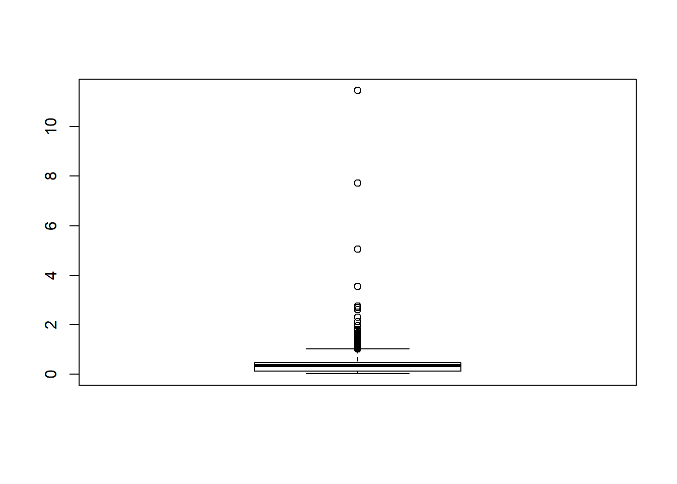

## model factors...
flist <- c('N1', 'N2', 'ICC_OV', 'ICC_LV', 'Estimator')
## Check assumptions
anova_assumptions_check(
  sdat, 'Estimate', factors = flist,
  model = as.formula('Estimate ~ N1 + N2 + ICC_OV + ICC_LV + Estimator + N1:N2 + N1:ICC_OV + N1:ICC_LV + N1:Estimator + N2:ICC_OV + N2:ICC_LV + N2:Estimator + ICC_OV:ICC_LV +  ICC_OV:Estimator  + ICC_LV:Estimator'))


 ============================= 

 Tests and Plots of Normality: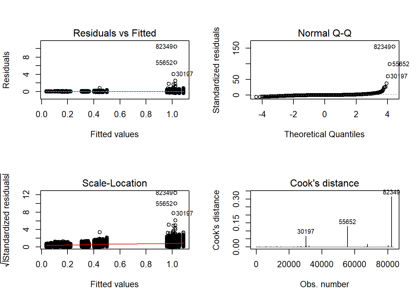


 Shapiro-Wilks Test of Normality of Residuals:

    Shapiro-Wilk normality test

data:  res
W = 0.8, p-value <2e-16


 K-S Test for Normality of Residuals:

    One-sample Kolmogorov-Smirnov test

data:  aov.out$residuals
D = 0.4, p-value <2e-16
alternative hypothesis: two-sided

`stat_bin()` using `bins = 30`. Pick better value with `binwidth`.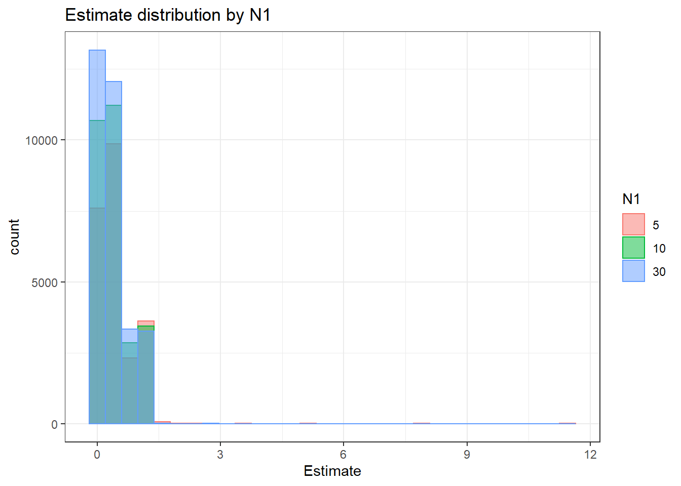

`stat_bin()` using `bins = 30`. Pick better value with `binwidth`.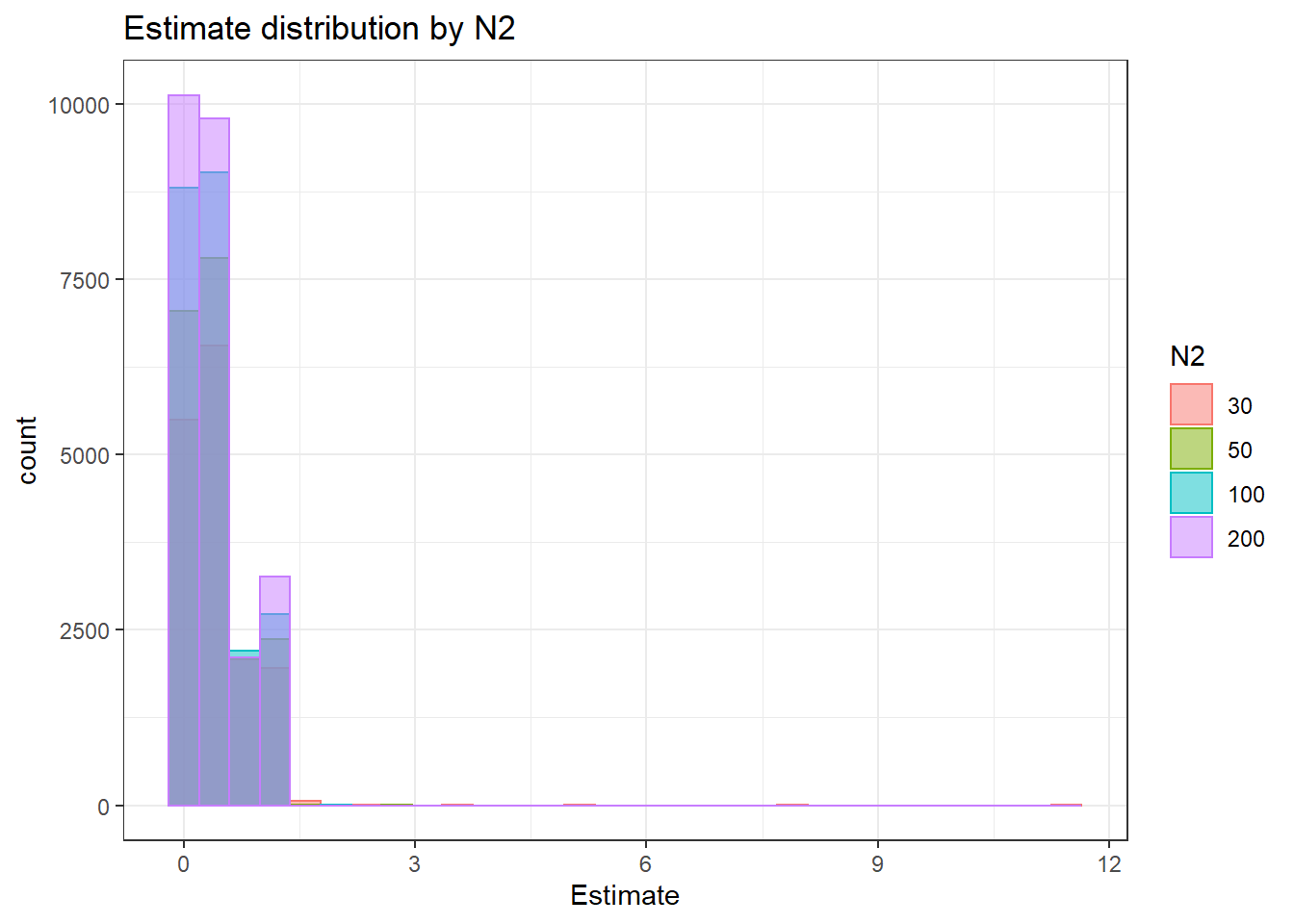

`stat_bin()` using `bins = 30`. Pick better value with `binwidth`.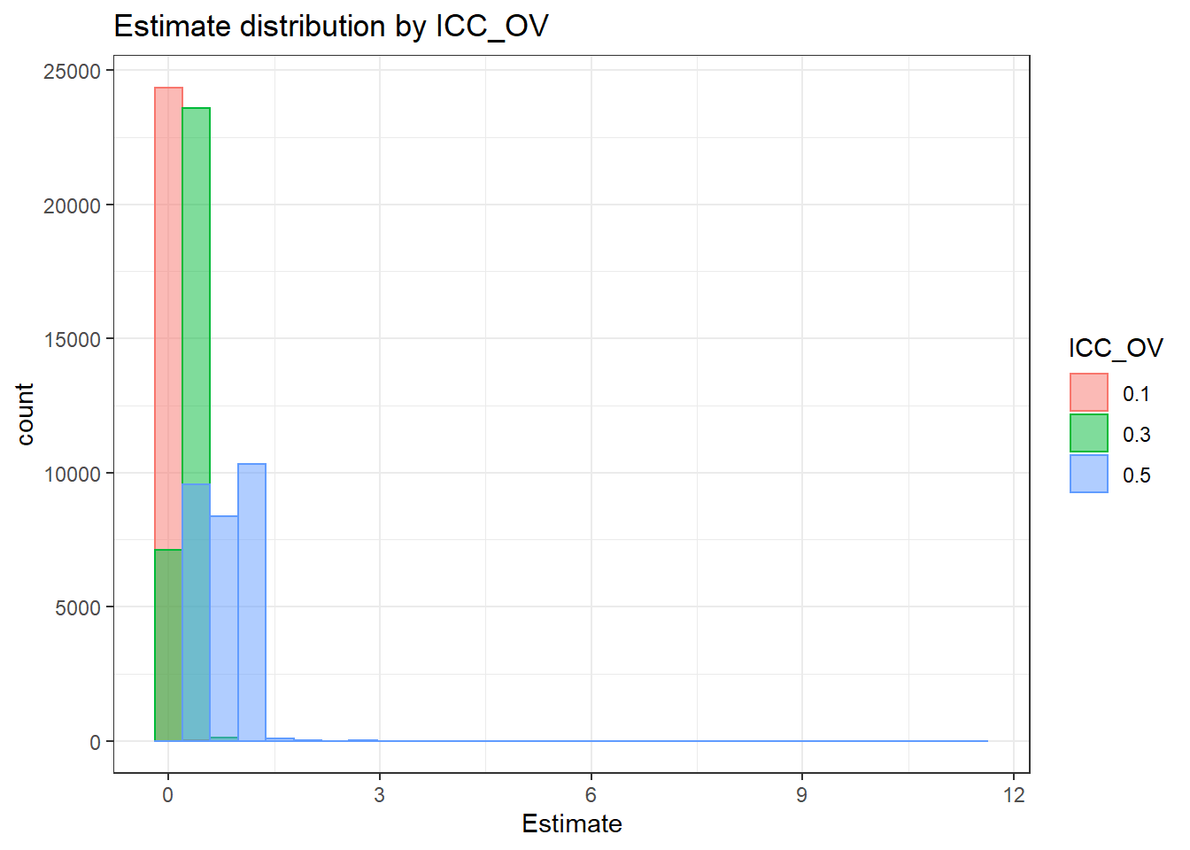

`stat_bin()` using `bins = 30`. Pick better value with `binwidth`.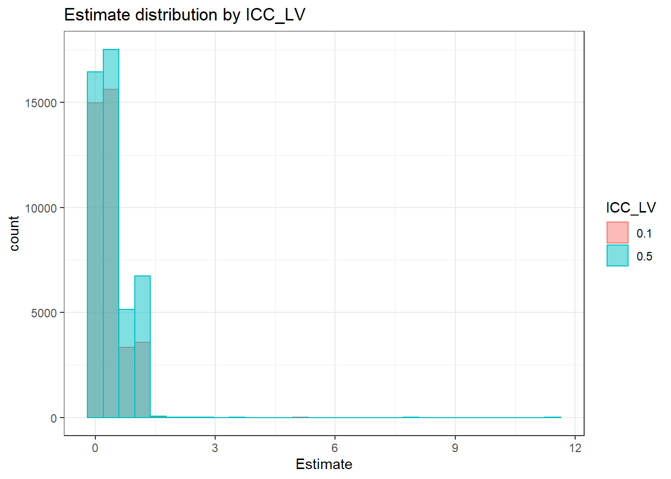

`stat_bin()` using `bins = 30`. Pick better value with `binwidth`.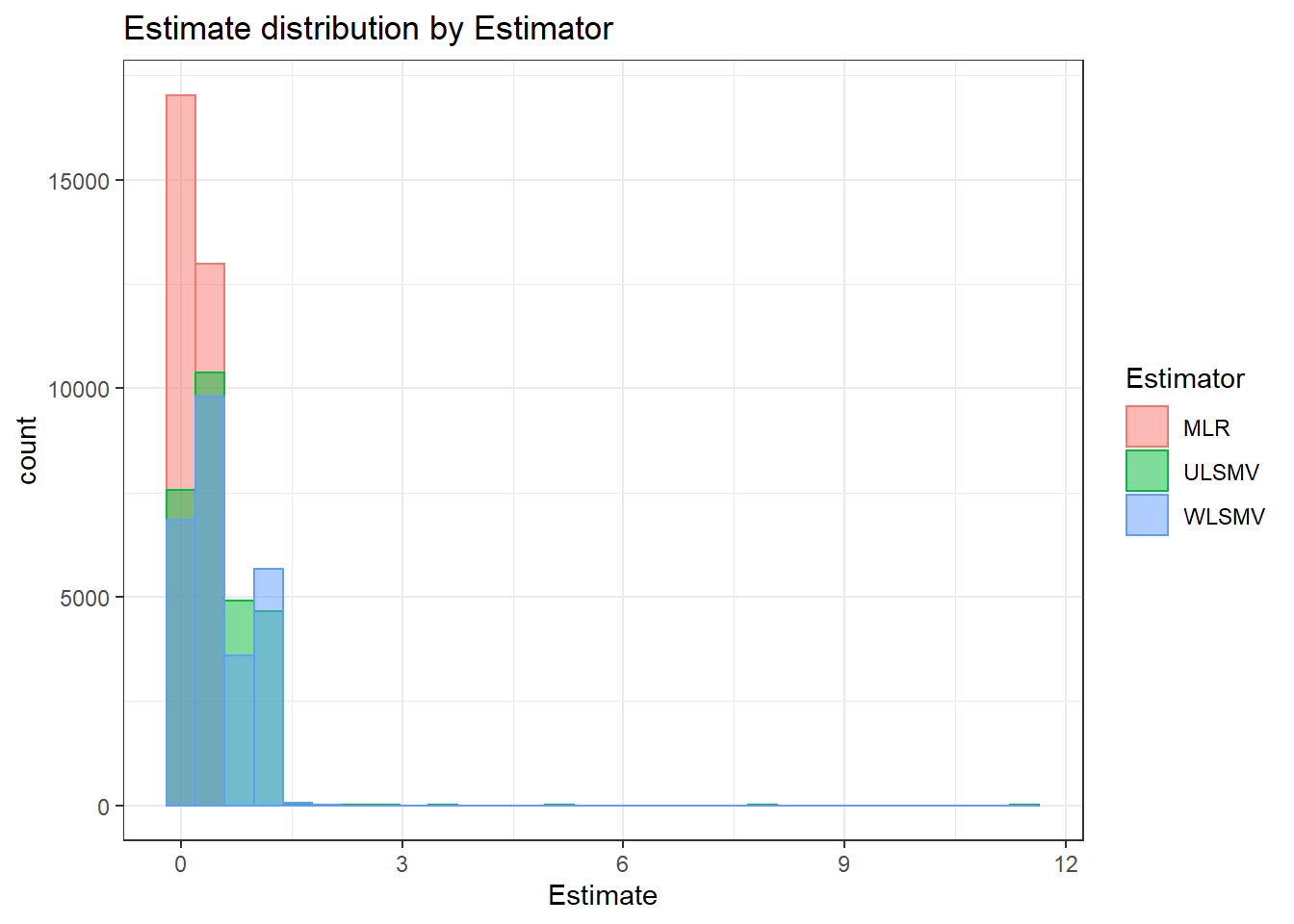


 ============================= 

 Tests of Homogeneity of Variance

 
 Levenes Test:  N1 
 
 
Levene's Test for Homogeneity of Variance (center = "mean")
         Df F value Pr(>F)    
group     2     136 <2e-16 ***
      83507                   
---
Signif. codes:  0 '***' 0.001 '**' 0.01 '*' 0.05 '.' 0.1 ' ' 1

 
 Levenes Test:  N2 
 
 
Levene's Test for Homogeneity of Variance (center = "mean")
         Df F value Pr(>F)    
group     3    51.4 <2e-16 ***
      83506                   
---
Signif. codes:  0 '***' 0.001 '**' 0.01 '*' 0.05 '.' 0.1 ' ' 1

 
 Levenes Test:  ICC_OV 
 
 
Levene's Test for Homogeneity of Variance (center = "mean")
         Df F value Pr(>F)    
group     2   58990 <2e-16 ***
      83507                   
---
Signif. codes:  0 '***' 0.001 '**' 0.01 '*' 0.05 '.' 0.1 ' ' 1

 
 Levenes Test:  ICC_LV 
 
 
Levene's Test for Homogeneity of Variance (center = "mean")
         Df F value Pr(>F)    
group     1     832 <2e-16 ***
      83508                   
---
Signif. codes:  0 '***' 0.001 '**' 0.01 '*' 0.05 '.' 0.1 ' ' 1

 
 Levenes Test:  Estimator 
 
 
Levene's Test for Homogeneity of Variance (center = "mean")
         Df F value Pr(>F)    
group     2   21534 <2e-16 ***
      83507                   
---
Signif. codes:  0 '***' 0.001 '**' 0.01 '*' 0.05 '.' 0.1 ' ' 1

ANOVA Results

model = as.formula('Estimate ~ N1 + N2 + ICC_OV + ICC_LV + Estimator + N1:N2 + N1:ICC_OV + N1:ICC_LV + N1:Estimator + N2:ICC_OV + N2:ICC_LV + N2:Estimator + ICC_OV:ICC_LV +  ICC_OV:Estimator  + ICC_LV:Estimator')

fit <- aov(model, data = sdat)
fit.out <- summary(fit)
fit.out

                    Df Sum Sq Mean Sq  F value  Pr(>F)    
N1                   2     61      31 6.73e+03 < 2e-16 ***
N2                   3     28       9 2.07e+03 < 2e-16 ***
ICC_OV               2   6341    3171 6.95e+05 < 2e-16 ***
ICC_LV               1      0       0 3.17e+01 1.8e-08 ***
Estimator            2   2060    1030 2.26e+05 < 2e-16 ***
N1:N2                6      3       1 1.24e+02 < 2e-16 ***
N1:ICC_OV            4      3       1 1.74e+02 < 2e-16 ***
N1:ICC_LV            2      0       0 3.37e+00   0.034 *  
N1:Estimator         4     18       4 9.73e+02 < 2e-16 ***
N2:ICC_OV            6      9       2 3.41e+02 < 2e-16 ***
N2:ICC_LV            3      1       0 8.41e+01 < 2e-16 ***
N2:Estimator         6     16       3 5.77e+02 < 2e-16 ***
ICC_OV:ICC_LV        2      3       2 3.82e+02 < 2e-16 ***
ICC_OV:Estimator     4   1163     291 6.37e+04 < 2e-16 ***
ICC_LV:Estimator     2      7       4 7.74e+02 < 2e-16 ***
Residuals        83460    381       0                     
---
Signif. codes:  0 '***' 0.001 '**' 0.01 '*' 0.05 '.' 0.1 ' ' 1

resultsList[["Level2-ResidualCovariance"]] <- cbind(omega2(fit.out), p_omega2(fit.out))
resultsList[["Level2-ResidualCovariance"]]

                 omega^2 partial-omega^2
N1                0.0061          0.1387
N2                0.0028          0.0693
ICC_OV            0.6281          0.9433
ICC_LV            0.0000          0.0004
Estimator         0.2040          0.8439
N1:N2             0.0003          0.0088
N1:ICC_OV         0.0003          0.0082
N1:ICC_LV         0.0000          0.0001
N1:Estimator      0.0018          0.0445
N2:ICC_OV         0.0009          0.0239
N2:ICC_LV         0.0001          0.0030
N2:Estimator      0.0016          0.0398
ICC_OV:ICC_LV     0.0003          0.0090
ICC_OV:Estimator  0.1152          0.7532
ICC_LV:Estimator  0.0007          0.0182

Summary Table of Effect Sizes

tb <- cbind(resultsList[[1]], resultsList[[2]], resultsList[[3]], resultsList[[4]])

kable(tb, format='html') %>%
    kable_styling(full_width = T) %>%
    add_header_above(c('Effect'=1,'Factor Loadings'=2,'Level-1 Factor Covariance'=2,'Level-2 Factor (co)variance'=2,'Level-2 Item Residual Variance'=2))

Effect	Factor Loadings		Level-1 Factor Covariance		Level-2 Factor (co)variance		Level-2 Item Residual Variance
	omega^2	partial-omega^2	omega^2	partial-omega^2	omega^2	partial-omega^2	omega^2	partial-omega^2
N1	0.000	0.002	0.000	0.000	0.003	0.018	0.006	0.139
N2	0.002	0.006	0.000	0.000	0.005	0.029	0.003	0.069
ICC_OV	0.008	0.030	0.000	0.000	0.022	0.122	0.628	0.943
ICC_LV	0.006	0.021	0.001	0.001	0.803	0.835	0.000	0.000
Estimator	0.700	0.726	0.000	0.000	0.003	0.019	0.204	0.844
N1:N2	0.000	0.000	0.000	0.000	0.000	0.001	0.000	0.009
N1:ICC_OV	0.000	0.000	0.000	0.000	0.000	0.000	0.000	0.008
N1:ICC_LV	0.000	0.000	0.000	0.000	0.000	0.000	0.000	0.000
N1:Estimator	0.001	0.002	0.000	0.000	0.000	0.002	0.002	0.044
N2:ICC_OV	0.000	0.001	0.000	0.000	0.000	0.001	0.001	0.024
N2:ICC_LV	0.000	0.000	0.000	0.000	0.001	0.004	0.000	0.003
N2:Estimator	0.001	0.003	0.000	0.000	0.002	0.014	0.002	0.040
ICC_OV:ICC_LV	0.000	0.001	0.000	0.000	0.000	0.001	0.000	0.009
ICC_OV:Estimator	0.015	0.053	0.000	0.000	0.000	0.003	0.115	0.753
ICC_LV:Estimator	0.004	0.014	0.000	0.000	0.001	0.006	0.001	0.018

## Print out in tex
print(xtable(tb, digits = 3), booktabs = T, include.rownames = T)

% latex table generated in R 3.6.3 by xtable 1.8-4 package
% Wed Jun 10 19:37:06 2020
\begin{table}[ht]
\centering
\begin{tabular}{rrrrrrrrr}
  \toprule
 & omega\verb|^|2 & partial-omega\verb|^|2 & omega\verb|^|2 & partial-omega\verb|^|2 & omega\verb|^|2 & partial-omega\verb|^|2 & omega\verb|^|2 & partial-omega\verb|^|2 \\ 
  \midrule
N1               & 0.000 & 0.002 & 0.000 & 0.000 & 0.003 & 0.018 & 0.006 & 0.139 \\ 
  N2               & 0.002 & 0.006 & 0.000 & 0.000 & 0.005 & 0.029 & 0.003 & 0.069 \\ 
  ICC\_OV           & 0.008 & 0.030 & 0.000 & 0.000 & 0.022 & 0.122 & 0.628 & 0.943 \\ 
  ICC\_LV           & 0.006 & 0.021 & 0.001 & 0.001 & 0.803 & 0.835 & 0.000 & 0.000 \\ 
  Estimator        & 0.700 & 0.726 & 0.000 & 0.000 & 0.003 & 0.019 & 0.204 & 0.844 \\ 
  N1:N2            & 0.000 & 0.000 & -0.000 & -0.000 & 0.000 & 0.001 & 0.000 & 0.009 \\ 
  N1:ICC\_OV        & 0.000 & 0.000 & 0.000 & 0.000 & 0.000 & 0.000 & 0.000 & 0.008 \\ 
  N1:ICC\_LV        & 0.000 & 0.000 & 0.000 & 0.000 & 0.000 & 0.000 & 0.000 & 0.000 \\ 
  N1:Estimator     & 0.001 & 0.002 & 0.000 & 0.000 & 0.000 & 0.002 & 0.002 & 0.044 \\ 
  N2:ICC\_OV        & 0.000 & 0.001 & -0.000 & -0.000 & 0.000 & 0.001 & 0.001 & 0.024 \\ 
  N2:ICC\_LV        & 0.000 & 0.000 & 0.000 & 0.000 & 0.001 & 0.004 & 0.000 & 0.003 \\ 
  N2:Estimator     & 0.001 & 0.003 & 0.000 & 0.000 & 0.002 & 0.014 & 0.002 & 0.040 \\ 
  ICC\_OV:ICC\_LV    & 0.000 & 0.001 & 0.000 & 0.000 & 0.000 & 0.001 & 0.000 & 0.009 \\ 
  ICC\_OV:Estimator & 0.015 & 0.053 & 0.000 & 0.000 & 0.000 & 0.003 & 0.115 & 0.753 \\ 
  ICC\_LV:Estimator & 0.004 & 0.014 & 0.000 & 0.000 & 0.001 & 0.006 & 0.001 & 0.018 \\ 
   \bottomrule
\end{tabular}
\end{table}

# ## Table of partial-omega2
# tb <- cbind(resultsList[[1]][,1, drop=F], resultsList[[2]][,1, drop=F], resultsList[[3]][,1, drop=F], resultsList[[4]][,1, drop=F])
# 
# kable(tb, format='html') %>%
#     kable_styling(full_width = T) %>%
#     add_header_above(c('Effect'=1,'Factor Loadings'=1,'Level-1 Factor Covariance'=1,'Level-2 Factor (co)variance'=2,'Level-2 Item Residual Variance'=2))
# 
# ## Print out in tex
# print(xtable(tb, digits = 3), booktabs = T, include.rownames = T)
# 
# 
# ## Table of omega-2
# tb <- cbind(resultsList[[1]][,1, drop=F], resultsList[[2]][,1, drop=F], resultsList[[3]][,1, drop=F], resultsList[[4]][,1, drop=F])
# 
# kable(tb, format='html') %>%
#     kable_styling(full_width = T) %>%
#     add_header_above(c('Effect'=1,'Factor Loadings'=2,'Level-1 Factor Covariance'=2,'Level-2 Factor (co)variance'=2,'Level-2 Item Residual Variance'=2))
# 
# ## Print out in tex
# print(xtable(tb, digits = 3), booktabs = T, include.rownames = T)

sessionInfo()

R version 3.6.3 (2020-02-29)
Platform: x86_64-w64-mingw32/x64 (64-bit)
Running under: Windows 10 x64 (build 18362)

Matrix products: default

locale:
[1] LC_COLLATE=English_United States.1252 
[2] LC_CTYPE=English_United States.1252   
[3] LC_MONETARY=English_United States.1252
[4] LC_NUMERIC=C                          
[5] LC_TIME=English_United States.1252    

attached base packages:
[1] stats     graphics  grDevices utils     datasets  methods   base     

other attached packages:
 [1] xtable_1.8-4          kableExtra_1.1.0      cowplot_1.0.0        
 [4] MplusAutomation_0.7-3 data.table_1.12.8     patchwork_1.0.0      
 [7] forcats_0.5.0         stringr_1.4.0         dplyr_0.8.5          
[10] purrr_0.3.4           readr_1.3.1           tidyr_1.1.0          
[13] tibble_3.0.1          ggplot2_3.3.0         tidyverse_1.3.0      
[16] workflowr_1.6.2      

loaded via a namespace (and not attached):
 [1] nlme_3.1-144      fs_1.4.1          lubridate_1.7.8   webshot_0.5.2    
 [5] httr_1.4.1        rprojroot_1.3-2   tools_3.6.3       backports_1.1.7  
 [9] R6_2.4.1          DBI_1.1.0         colorspace_1.4-1  withr_2.2.0      
[13] tidyselect_1.1.0  curl_4.3          compiler_3.6.3    git2r_0.27.1     
[17] cli_2.0.2         rvest_0.3.5       xml2_1.3.2        labeling_0.3     
[21] scales_1.1.1      digest_0.6.25     foreign_0.8-75    rmarkdown_2.1    
[25] rio_0.5.16        pkgconfig_2.0.3   htmltools_0.4.0   highr_0.8        
[29] dbplyr_1.4.4      rlang_0.4.6       readxl_1.3.1      rstudioapi_0.11  
[33] generics_0.0.2    farver_2.0.3      jsonlite_1.6.1    zip_2.0.4        
[37] car_3.0-8         magrittr_1.5      texreg_1.36.23    Rcpp_1.0.4.6     
[41] munsell_0.5.0     fansi_0.4.1       abind_1.4-5       proto_1.0.0      
[45] lifecycle_0.2.0   stringi_1.4.6     yaml_2.2.1        carData_3.0-4    
[49] plyr_1.8.6        grid_3.6.3        blob_1.2.1        parallel_3.6.3   
[53] promises_1.1.0    crayon_1.3.4      lattice_0.20-38   haven_2.3.0      
[57] pander_0.6.3      hms_0.5.3         knitr_1.28        pillar_1.4.4     
[61] boot_1.3-24       reprex_0.3.0      glue_1.4.1        evaluate_0.14    
[65] modelr_0.1.8      vctrs_0.3.0       httpuv_1.5.2      cellranger_1.1.0 
[69] gtable_0.3.0      assertthat_0.2.1  gsubfn_0.7        xfun_0.14        
[73] openxlsx_4.1.5    broom_0.5.6       coda_0.19-3       later_1.0.0      
[77] viridisLite_0.3.0 ellipsis_0.3.1

Design Effects on Parameter Estimates

2020-06-01

Packages and Set-Up

Data Management

ANOVA and effect sizes for distributional differences

Factor Loadings

Assumption Checking

ANOVA Results

Level-1 factor Covariance

Assumption Checking

ANOVA Results

Level-2 factor (co)variances

Assumption Checking

ANOVA Results

Level-2 item residual variances

Assumption Checking

ANOVA Results

Summary Table of Effect Sizes