Last updated: 2020-06-10

Checks: 6 1

Knit directory: mcfa-para-est/

This reproducible R Markdown analysis was created with workflowr (version 1.6.2). The Checks tab describes the reproducibility checks that were applied when the results were created. The Past versions tab lists the development history.

R Markdown file: uncommitted changes

The R Markdown is untracked by Git. To know which version of the R Markdown file created these results, you’ll want to first commit it to the Git repo. If you’re still working on the analysis, you can ignore this warning. When you’re finished, you can run wflow_publish to commit the R Markdown file and build the HTML.

Environment: empty

Great job! The global environment was empty. Objects defined in the global environment can affect the analysis in your R Markdown file in unknown ways. For reproduciblity it’s best to always run the code in an empty environment.

Seed: set.seed(20190614)

The command set.seed(20190614) was run prior to running the code in the R Markdown file. Setting a seed ensures that any results that rely on randomness, e.g. subsampling or permutations, are reproducible.

Session information: recorded

Great job! Recording the operating system, R version, and package versions is critical for reproducibility.

Cache: none

Nice! There were no cached chunks for this analysis, so you can be confident that you successfully produced the results during this run.

File paths: relative

Great job! Using relative paths to the files within your workflowr project makes it easier to run your code on other machines.

Repository version: eecb366

Great! You are using Git for version control. Tracking code development and connecting the code version to the results is critical for reproducibility.

The results in this page were generated with repository version eecb366. See the Past versions tab to see a history of the changes made to the R Markdown and HTML files.

Note that you need to be careful to ensure that all relevant files for the analysis have been committed to Git prior to generating the results (you can use wflow_publish or wflow_git_commit). workflowr only checks the R Markdown file, but you know if there are other scripts or data files that it depends on. Below is the status of the Git repository when the results were generated:


Ignored files:
    Ignored:    .Rhistory
    Ignored:    .Rproj.user/
    Ignored:    data/compiled_para_results.txt
    Ignored:    data/results_bias_est.csv
    Ignored:    data/results_bias_se.csv
    Ignored:    fig/
    Ignored:    manuscript/
    Ignored:    output/fact-cov-converge-largeN.pdf
    Ignored:    output/fact-cov-converge-medN.pdf
    Ignored:    output/fact-cov-converge-smallN.pdf
    Ignored:    output/loading-converge-largeN.pdf
    Ignored:    output/loading-converge-medN.pdf
    Ignored:    output/loading-converge-smallN.pdf
    Ignored:    references/
    Ignored:    sera-presentation/

Untracked files:
    Untracked:  analysis/ml-cfa-parameter-anova-estimates.Rmd
    Untracked:  analysis/ml-cfa-parameter-anova-relative-bias.Rmd
    Untracked:  analysis/ml-cfa-parameter-bias-latent-ICC.Rmd
    Untracked:  analysis/ml-cfa-parameter-bias-observed-ICC.Rmd
    Untracked:  analysis/ml-cfa-parameter-bias-pub-figure.Rmd
    Untracked:  analysis/ml-cfa-parameter-convergence-ARD-L1-factor-covariance.Rmd
    Untracked:  analysis/ml-cfa-parameter-convergence-ARD-L2-factor-covariance.Rmd
    Untracked:  analysis/ml-cfa-parameter-convergence-ARD-L2-factor-variance.Rmd
    Untracked:  analysis/ml-cfa-parameter-convergence-ARD-L2-residual-variance.Rmd
    Untracked:  analysis/ml-cfa-parameter-convergence-ARD-factor-loadings.Rmd
    Untracked:  analysis/ml-cfa-parameter-convergence-ARD-latent-ICC.Rmd
    Untracked:  analysis/ml-cfa-parameter-convergence-ARD-observed-ICC.Rmd
    Untracked:  analysis/ml-cfa-parameter-convergence-correlation-pubfigure.Rmd
    Untracked:  analysis/ml-cfa-parameter-convergence-trace-plots-factor-loadings.Rmd
    Untracked:  analysis/ml-cfa-standard-error-anova-logSE.Rmd
    Untracked:  analysis/ml-cfa-standard-error-anova-relative-bias.Rmd
    Untracked:  analysis/ml-cfa-standard-error-bias-factor-loadings.Rmd
    Untracked:  analysis/ml-cfa-standard-error-bias-level1-factor-covariances.Rmd
    Untracked:  analysis/ml-cfa-standard-error-bias-level2-factor-covariances.Rmd
    Untracked:  analysis/ml-cfa-standard-error-bias-level2-factor-variances.Rmd
    Untracked:  analysis/ml-cfa-standard-error-bias-level2-residual-variances.Rmd
    Untracked:  analysis/ml-cfa-standard-error-bias-overview.Rmd
    Untracked:  code/r_functions.R
    Untracked:  renv.lock
    Untracked:  renv/

Unstaged changes:
    Modified:   .gitignore
    Modified:   analysis/index.Rmd
    Modified:   analysis/ml-cfa-convergence-summary.Rmd
    Modified:   analysis/ml-cfa-parameter-bias-factor-loadings.Rmd
    Modified:   analysis/ml-cfa-parameter-bias-level1-factor-covariances.Rmd
    Modified:   analysis/ml-cfa-parameter-bias-level2-factor-covariances.Rmd
    Modified:   analysis/ml-cfa-parameter-bias-level2-factor-variances.Rmd
    Modified:   analysis/ml-cfa-parameter-bias-level2-residual-variances.Rmd
    Modified:   analysis/ml-cfa-parameter-convergence-correlation-factor-loadings.Rmd
    Modified:   code/get_data.R
    Modified:   code/load_packages.R

Note that any generated files, e.g. HTML, png, CSS, etc., are not included in this status report because it is ok for generated content to have uncommitted changes.

There are no past versions. Publish this analysis with wflow_publish() to start tracking its development.

The purpose of this page is to identify the impact of design factors on standard error estimates. This is done using analysis of variance (factorial) on the estimates of relative bias (RB) for the estimated parameter.

Packages and Set-Up

rm(list=ls())
source(paste0(getwd(),"/code/load_packages.R"))
source(paste0(getwd(),"/code/get_data.R"))
source(paste0(getwd(),"/code/r_functions.R"))

# general options
theme_set(theme_bw())
options(digits=3)

##Chunk iptions
knitr::opts_chunk$set(out.width="225%")

Data Management

# set up vectors of variable names
pvec <- c(paste0('lambda1',1:6), paste0('lambda2',6:10), 'psiW12','psiB1', 'psiB2', 'psiB12', paste0('thetaB',1:10), 'icc_lv1_est', 'icc_lv2_est', paste0('icc_ov',1:10,'_est'))
# stored "true" values of parameters by each condition
ptvec <- c(rep('lambdaT',11), 'psiW12T', 'psiB1T', 'psiB2T', 'psiB12T', rep("thetaBT", 10), rep('icc_lv',2), rep('icc_ov',10))


# take out non-converged/inadmissible cases
sim_results <- filter(sim_results, Converge==1, Admissible==1)

# Set conditions levels as categorical values
sim_results <- sim_results %>%
  mutate(N1 = factor(N1, c("5", "10", "30")),
         N2 = factor(N2, c("30", "50", "100", "200")),
         ICC_OV = factor(ICC_OV, c("0.1","0.3", "0.5")),
         ICC_LV = factor(ICC_LV, c("0.1", "0.5")))

# convert to long format
long_res1 <- sim_results[,c("Condition", "Replication", "N1", "N2", "ICC_OV", "ICC_LV", "Estimator", pvec)] %>%
  pivot_longer(
    cols = all_of(pvec),
    names_to = "Parameter",
    values_to = "Estimate"
  )

long_res2 <- tibble(sim_results[,c("Condition", "Replication", "N1", "N2", "ICC_OV", "ICC_LV", "Estimator", ptvec)], .name_repair="universal")
ptvec <- colnames(long_res2)[8:44]
long_res2 <- long_res2 %>%
  pivot_longer(
    cols = all_of(ptvec),
    names_to = "ParameterT",
    values_to = "Truth"
  )

long_results <- long_res1
long_results$ParameterT <- long_res2$ParameterT
long_results$Truth <- long_res2$Truth

Now, we are only going to do ANOVA on the relative bias estimates (RB).

long_results <- long_results %>%
  mutate(RB = ((Estimate - Truth))/Truth*100)


# Object to Story Results
resultsList <- list()

ANOVA and effect sizes for distributional differences

For this simulation experiment, there were 5 factors systematically varied. Of these 5 factors, 4 were factors influencing the observed data and 1 were factors pertaining to estimation and model fitting. The factors were

Level-1 sample size (5, 10, 30)
Level-2 sample size (30, 50, 100, 200)
Observed indicator ICC (.1, .3, .5)
Latent variable ICC (.1, .5)
Model estimator (MLR, ULSMV, WLSMV)

For each parameter, an analysis of variance (ANOVA) was conducted in order to test how much influence each of these design factors.

General Linear Model investigated for estimated parameter was: \[ Y_{ijklmn} = \mu + \alpha_{j} + \beta_{k} + \gamma_{l} + \delta_m + \theta_n +\\ (\alpha\beta)_{jk} + (\alpha\gamma)_{jl}+ (\alpha\delta)_{jm} + (\alpha\theta)_{jn}+ \\ (\beta\gamma)_{kl}+ (\beta\delta)_{km} + (\beta\theta)_{kn}+ (\gamma\delta)_{lm} + + (\gamma\theta)_{ln} + (\delta\theta)_{mn} + \varepsilon_{ijklmn} \] where

\(\mu\) is the grand mean,
\(\alpha_{j}\) is the effect of Level-1 sample size,
\(\beta_{k}\) is the effect of Level-2 sample size,
\(\gamma_{l}\) is the effect of Observed indicator ICC,
\(\delta_m\) is the effect of Latent variable ICC,
\(\theta_n\) is the effect of Model estimator ,
\((\alpha\beta)_{jk}\) is the interaction between Level-1 sample size and Level-2 sample size,
\((\alpha\gamma)_{jl}\) is the interaction between Level-1 sample size and Observed indicator ICC,
\((\alpha\delta)_{jm}\) is the interaction between Level-1 sample size and Latent variable ICC,
\((\alpha\theta)_{jn}\) is the interaction between Level-1 sample size and Model estimator ,
\((\beta\gamma)_{kl}\) is the interaction between Level-2 sample size and Observed indicator ICC,
\((\beta\delta)_{km}\) is the interaction between Level-2 sample size and Latent variable ICC,
\((\beta\theta)_{kn}\) is the interaction between Level-2 sample size and Model estimator ,
\((\gamma\delta)_{lm}\) is the interaction between Observed indicator ICC and Latent variable ICC,
\((\gamma\theta)_{ln}\) is the interaction between Observed indicator ICC and Model estimator ,
\((\delta\theta)_{mn}\) is the interaction between Latent variable ICC and Model estimator , and
\(\varepsilon_{ijklmn}\) is the residual error for the \(i^{th}\) observed SE estimate.

Note that for most of these terms there are actually 2 or 3 terms actually estimated. These additional terms are because of the categorical nature of each effect so we have to create “reference” groups and calculate the effect of being in a group other than the reference group. Higher order interactions were omitted for clarity of interpretation of the model. If interested in higher-order interactions, please see Maxwell and Delaney (2004).

The real reason the higher order interaction was omitted: Because I have no clue how to interpret a 5-way interaction (whatever the heck that is), I am limiting the ANOVA to all bivariate interactions.

Diagnostics for factorial ANOVA:

Independence of Observations
Normality of residuals across cells for the design
Homogeneity of variance across cells

Independence of observations is by design, where these data were randomly generated from a known population and observations are across replications and are independent. The normality assumptions is that the residuals of the models are normally distributed across the design cells. The normality assumption is tested by investigation by Shapiro-Wilks Test, the K-S test, and visual inspection of QQ-plots and histograms. The equality of variance is checked through Levene’s test across all the different conditions/groupings. Furthermore, the plots of the residuals are also indicative of the equality of variance across groups as there should be no apparent pattern to the residual plots.

Factor Loadings

Assumption Checking

sdat <- filter(long_results, Parameter %like% "lambda")

sdat <- sdat %>%
  group_by(Replication, N1, N2, ICC_OV, ICC_LV, Estimator) %>%
  summarise(RB = mean(RB))

# first, look at summary of RB Estimates
boxplot(sdat$RB)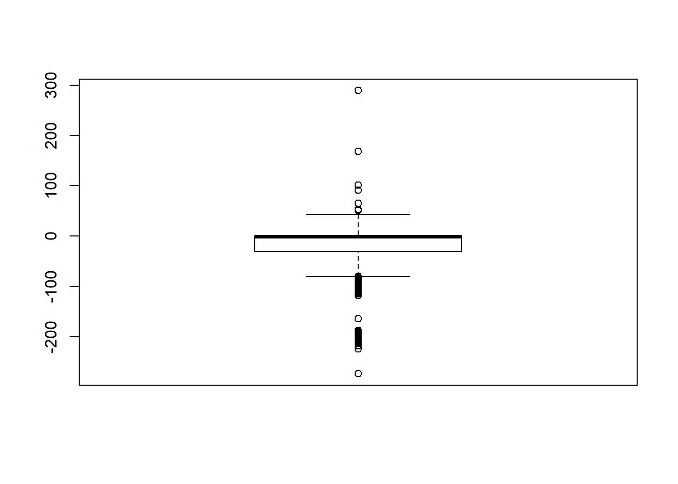

## model factors...
flist <- c('N1', 'N2', 'ICC_OV', 'ICC_LV', 'Estimator')
## Check assumptions
anova_assumptions_check(
  sdat, 'RB', factors = flist,
  model = as.formula('RB ~ N1 + N2 + ICC_OV + ICC_LV + Estimator + N1:N2 + N1:ICC_OV + N1:ICC_LV + N1:Estimator + N2:ICC_OV + N2:ICC_LV + N2:Estimator + ICC_OV:ICC_LV +  ICC_OV:Estimator  + ICC_LV:Estimator'))


 ============================= 

 Tests and Plots of Normality: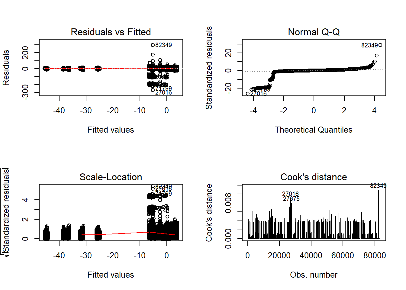


 Shapiro-Wilks Test of Normality of Residuals:

    Shapiro-Wilk normality test

data:  res
W = 0.3, p-value <2e-16


 K-S Test for Normality of Residuals:

    One-sample Kolmogorov-Smirnov test

data:  aov.out$residuals
D = 0.3, p-value <2e-16
alternative hypothesis: two-sided

`stat_bin()` using `bins = 30`. Pick better value with `binwidth`.

Warning: Removed 254 rows containing non-finite values (stat_bin).

Warning: Removed 3 rows containing missing values (geom_bar).

`stat_bin()` using `bins = 30`. Pick better value with `binwidth`.

Warning: Removed 254 rows containing non-finite values (stat_bin).

Warning: Removed 4 rows containing missing values (geom_bar).

`stat_bin()` using `bins = 30`. Pick better value with `binwidth`.

Warning: Removed 254 rows containing non-finite values (stat_bin).

Warning: Removed 3 rows containing missing values (geom_bar).

`stat_bin()` using `bins = 30`. Pick better value with `binwidth`.

Warning: Removed 254 rows containing non-finite values (stat_bin).

Warning: Removed 2 rows containing missing values (geom_bar).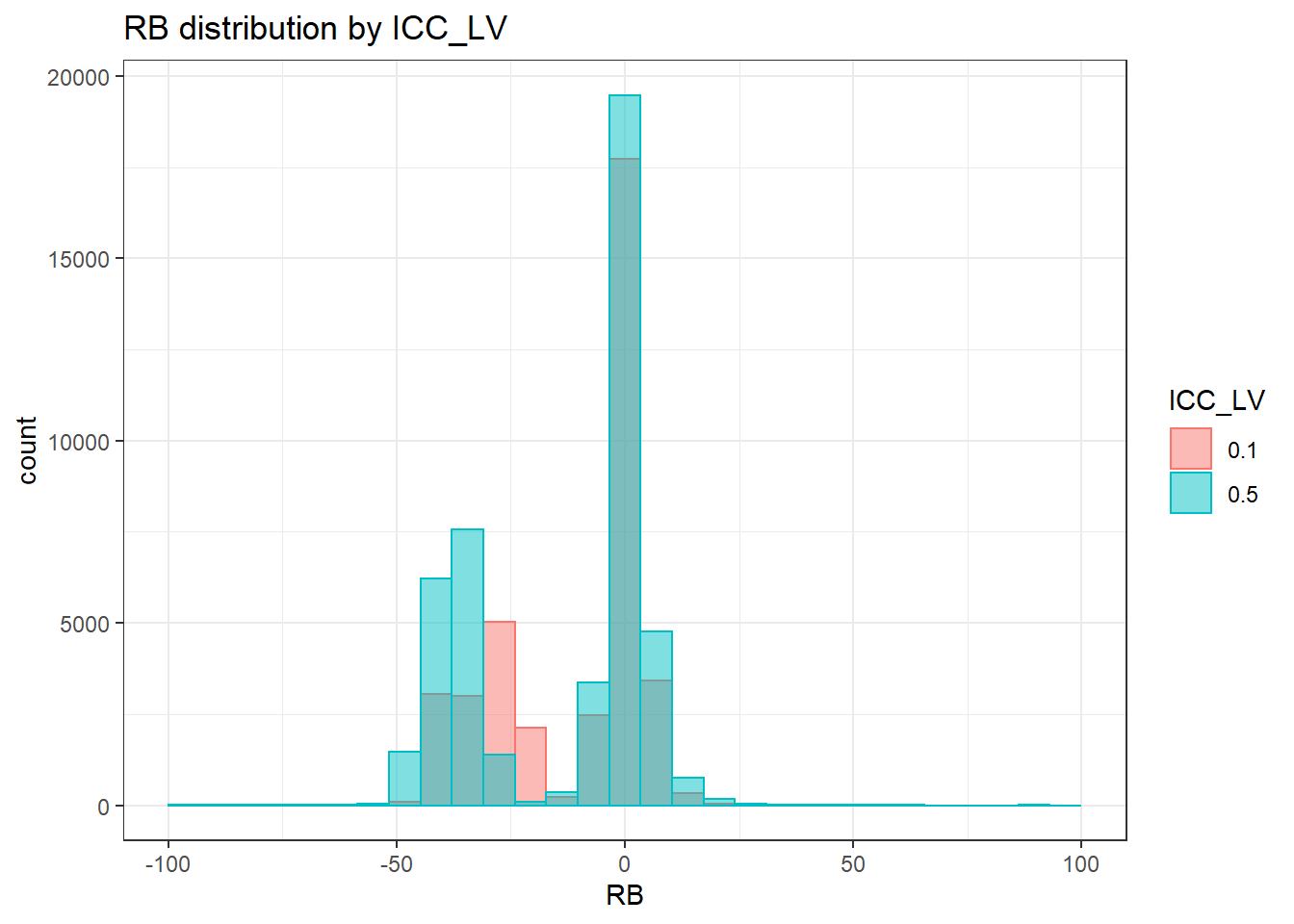

`stat_bin()` using `bins = 30`. Pick better value with `binwidth`.

Warning: Removed 254 rows containing non-finite values (stat_bin).

Warning: Removed 3 rows containing missing values (geom_bar).


 ============================= 

 Tests of Homogeneity of Variance

 
 Levenes Test:  N1 
 
 
Levene's Test for Homogeneity of Variance (center = "mean")
         Df F value Pr(>F)    
group     2     206 <2e-16 ***
      83507                   
---
Signif. codes:  0 '***' 0.001 '**' 0.01 '*' 0.05 '.' 0.1 ' ' 1

 
 Levenes Test:  N2 
 
 
Levene's Test for Homogeneity of Variance (center = "mean")
         Df F value Pr(>F)    
group     3     216 <2e-16 ***
      83506                   
---
Signif. codes:  0 '***' 0.001 '**' 0.01 '*' 0.05 '.' 0.1 ' ' 1

 
 Levenes Test:  ICC_OV 
 
 
Levene's Test for Homogeneity of Variance (center = "mean")
         Df F value Pr(>F)    
group     2    3722 <2e-16 ***
      83507                   
---
Signif. codes:  0 '***' 0.001 '**' 0.01 '*' 0.05 '.' 0.1 ' ' 1

 
 Levenes Test:  ICC_LV 
 
 
Levene's Test for Homogeneity of Variance (center = "mean")
         Df F value Pr(>F)    
group     1    3934 <2e-16 ***
      83508                   
---
Signif. codes:  0 '***' 0.001 '**' 0.01 '*' 0.05 '.' 0.1 ' ' 1

 
 Levenes Test:  Estimator 
 
 
Levene's Test for Homogeneity of Variance (center = "mean")
         Df F value Pr(>F)    
group     2     560 <2e-16 ***
      83507                   
---
Signif. codes:  0 '***' 0.001 '**' 0.01 '*' 0.05 '.' 0.1 ' ' 1

# was bad... Remove extreme outliers
quantile(sdat$RB, c(0.001, 0.01, 0.99, 0.999))

  0.1%     1%    99%  99.9% 
-199.4  -46.5   12.3   23.3

# remove RB>100
sdat <- filter(sdat, RB <= 100)
boxplot(sdat$RB)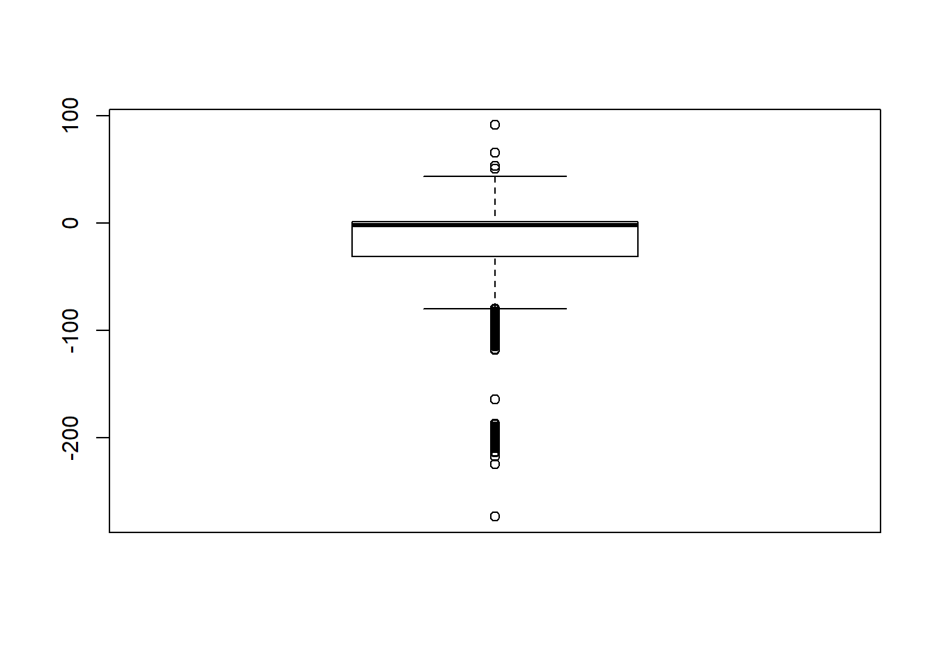

# rerun
## Check assumptions
anova_assumptions_check(
  sdat, 'RB', factors = flist,
  model = as.formula('RB ~ N1 + N2 + ICC_OV + ICC_LV + Estimator + N1:N2 + N1:ICC_OV + N1:ICC_LV + N1:Estimator + N2:ICC_OV + N2:ICC_LV + N2:Estimator + ICC_OV:ICC_LV +  ICC_OV:Estimator  + ICC_LV:Estimator'))


 ============================= 

 Tests and Plots of Normality: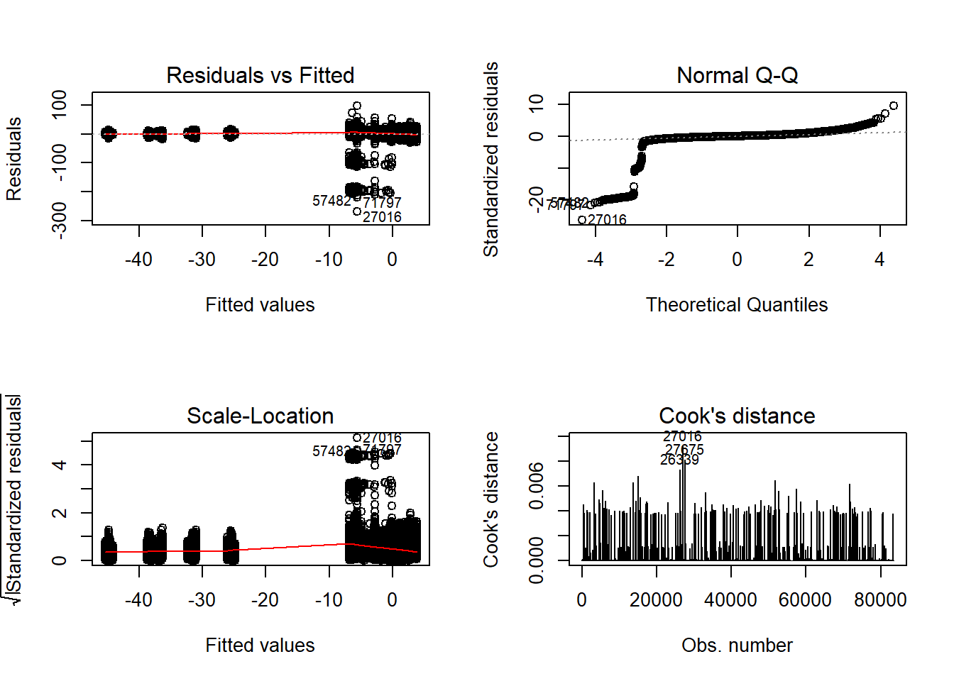


 Shapiro-Wilks Test of Normality of Residuals:

    Shapiro-Wilk normality test

data:  res
W = 0.3, p-value <2e-16


 K-S Test for Normality of Residuals:

    One-sample Kolmogorov-Smirnov test

data:  aov.out$residuals
D = 0.3, p-value <2e-16
alternative hypothesis: two-sided

`stat_bin()` using `bins = 30`. Pick better value with `binwidth`.

Warning: Removed 251 rows containing non-finite values (stat_bin).

Warning: Removed 3 rows containing missing values (geom_bar).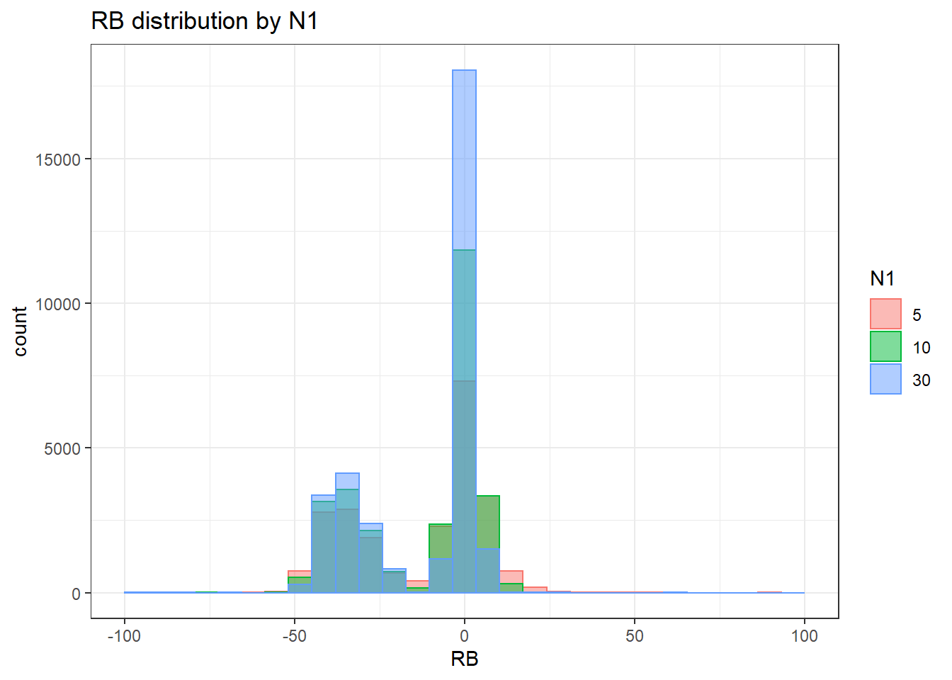

`stat_bin()` using `bins = 30`. Pick better value with `binwidth`.

Warning: Removed 251 rows containing non-finite values (stat_bin).

Warning: Removed 4 rows containing missing values (geom_bar).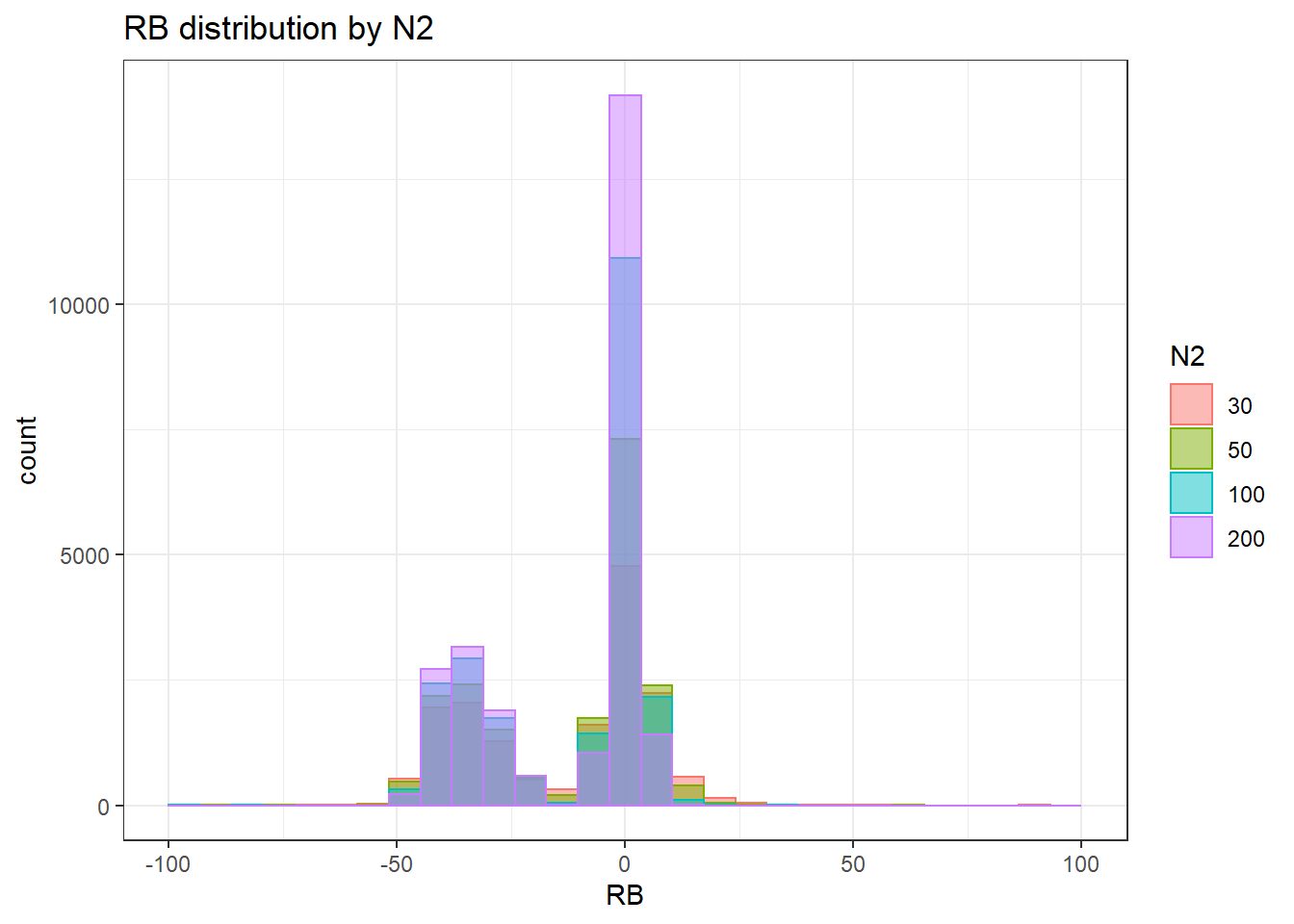

`stat_bin()` using `bins = 30`. Pick better value with `binwidth`.

Warning: Removed 251 rows containing non-finite values (stat_bin).

Warning: Removed 3 rows containing missing values (geom_bar).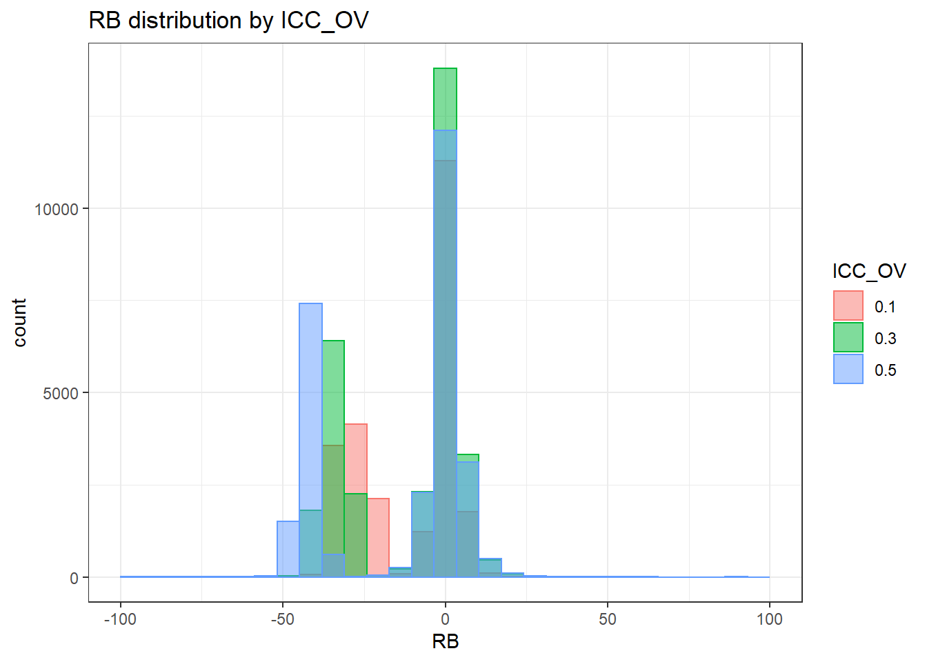

`stat_bin()` using `bins = 30`. Pick better value with `binwidth`.

Warning: Removed 251 rows containing non-finite values (stat_bin).

Warning: Removed 2 rows containing missing values (geom_bar).

`stat_bin()` using `bins = 30`. Pick better value with `binwidth`.

Warning: Removed 251 rows containing non-finite values (stat_bin).

Warning: Removed 3 rows containing missing values (geom_bar).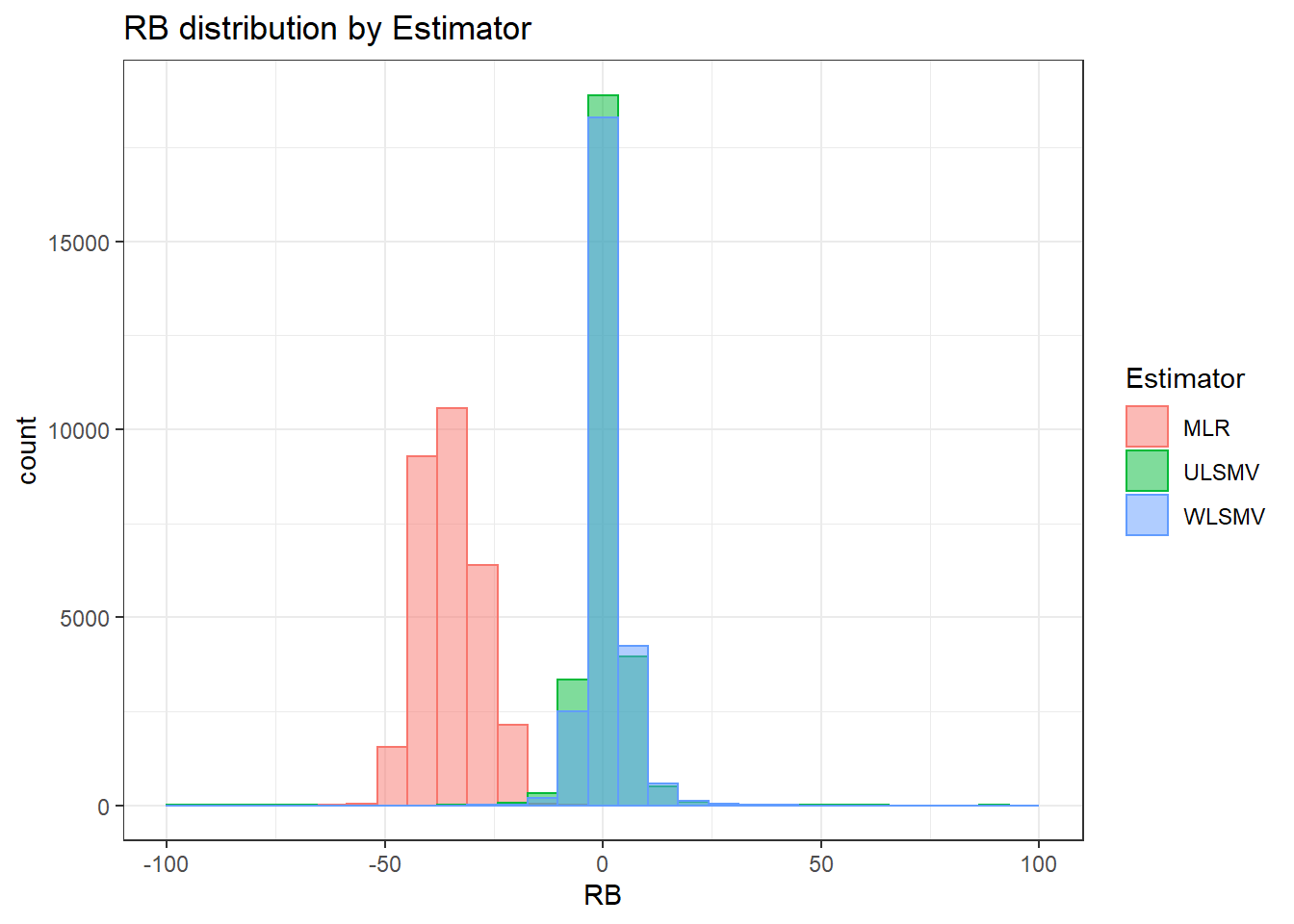


 ============================= 

 Tests of Homogeneity of Variance

 
 Levenes Test:  N1 
 
 
Levene's Test for Homogeneity of Variance (center = "mean")
         Df F value Pr(>F)    
group     2     204 <2e-16 ***
      83504                   
---
Signif. codes:  0 '***' 0.001 '**' 0.01 '*' 0.05 '.' 0.1 ' ' 1

 
 Levenes Test:  N2 
 
 
Levene's Test for Homogeneity of Variance (center = "mean")
         Df F value Pr(>F)    
group     3     215 <2e-16 ***
      83503                   
---
Signif. codes:  0 '***' 0.001 '**' 0.01 '*' 0.05 '.' 0.1 ' ' 1

 
 Levenes Test:  ICC_OV 
 
 
Levene's Test for Homogeneity of Variance (center = "mean")
         Df F value Pr(>F)    
group     2    3765 <2e-16 ***
      83504                   
---
Signif. codes:  0 '***' 0.001 '**' 0.01 '*' 0.05 '.' 0.1 ' ' 1

 
 Levenes Test:  ICC_LV 
 
 
Levene's Test for Homogeneity of Variance (center = "mean")
         Df F value Pr(>F)    
group     1    3981 <2e-16 ***
      83505                   
---
Signif. codes:  0 '***' 0.001 '**' 0.01 '*' 0.05 '.' 0.1 ' ' 1

 
 Levenes Test:  Estimator 
 
 
Levene's Test for Homogeneity of Variance (center = "mean")
         Df F value Pr(>F)    
group     2     567 <2e-16 ***
      83504                   
---
Signif. codes:  0 '***' 0.001 '**' 0.01 '*' 0.05 '.' 0.1 ' ' 1

ANOVA Results

model = as.formula('RB ~ N1 + N2 + ICC_OV + ICC_LV + Estimator + N1:N2 + N1:ICC_OV + N1:ICC_LV + N1:Estimator + N2:ICC_OV + N2:ICC_LV + N2:Estimator + ICC_OV:ICC_LV +  ICC_OV:Estimator  + ICC_LV:Estimator')

fit <- aov(model, data = sdat)
fit.out <- summary(fit)
fit.out

                    Df   Sum Sq  Mean Sq  F value  Pr(>F)    
N1                   2    18915     9458 9.15e+01 < 2e-16 ***
N2                   3    56697    18899 1.83e+02 < 2e-16 ***
ICC_OV               2   276510   138255 1.34e+03 < 2e-16 ***
ICC_LV               1   187369   187369 1.81e+03 < 2e-16 ***
Estimator            2 23237551 11618775 1.12e+05 < 2e-16 ***
N1:N2                6     2947      491 4.75e+00 7.6e-05 ***
N1:ICC_OV            4      742      186 1.79e+00    0.13    
N1:ICC_LV            2      221      110 1.07e+00    0.34    
N1:Estimator         4    20103     5026 4.86e+01 < 2e-16 ***
N2:ICC_OV            6     8628     1438 1.39e+01 7.1e-16 ***
N2:ICC_LV            3      442      147 1.43e+00    0.23    
N2:Estimator         6    27214     4536 4.39e+01 < 2e-16 ***
ICC_OV:ICC_LV        2     6794     3397 3.29e+01 5.5e-15 ***
ICC_OV:Estimator     4   492400   123100 1.19e+03 < 2e-16 ***
ICC_LV:Estimator     2   127886    63943 6.18e+02 < 2e-16 ***
Residuals        83457  8630321      103                     
---
Signif. codes:  0 '***' 0.001 '**' 0.01 '*' 0.05 '.' 0.1 ' ' 1

resultsList[["FactorLoadings"]] <- cbind(omega2(fit.out), p_omega2(fit.out))
resultsList[["FactorLoadings"]]

                 omega^2 partial-omega^2
N1                0.0006          0.0022
N2                0.0017          0.0065
ICC_OV            0.0083          0.0310
ICC_LV            0.0057          0.0212
Estimator         0.7021          0.7291
N1:N2             0.0001          0.0003
N1:ICC_OV         0.0000          0.0000
N1:ICC_LV         0.0000          0.0000
N1:Estimator      0.0006          0.0023
N2:ICC_OV         0.0002          0.0009
N2:ICC_LV         0.0000          0.0000
N2:Estimator      0.0008          0.0031
ICC_OV:ICC_LV     0.0002          0.0008
ICC_OV:Estimator  0.0149          0.0539
ICC_LV:Estimator  0.0039          0.0146

Level-1 factor Covariance

Assumption Checking

sdat <- filter(long_results, Parameter %like% "psiW")

sdat <- sdat %>%
  group_by(Replication, N1, N2, ICC_OV, ICC_LV, Estimator) %>%
  summarise(RB = mean(RB))

# first, look at summary of RB Estimates
boxplot(sdat$RB)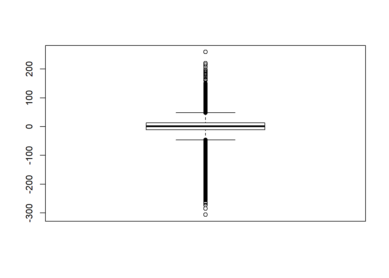

## model factors...
flist <- c('N1', 'N2', 'ICC_OV', 'ICC_LV', 'Estimator')
## Check assumptions
anova_assumptions_check(
  sdat, 'RB', factors = flist,
  model = as.formula('RB ~ N1 + N2 + ICC_OV + ICC_LV + Estimator + N1:N2 + N1:ICC_OV + N1:ICC_LV + N1:Estimator + N2:ICC_OV + N2:ICC_LV + N2:Estimator + ICC_OV:ICC_LV +  ICC_OV:Estimator  + ICC_LV:Estimator'))


 ============================= 

 Tests and Plots of Normality: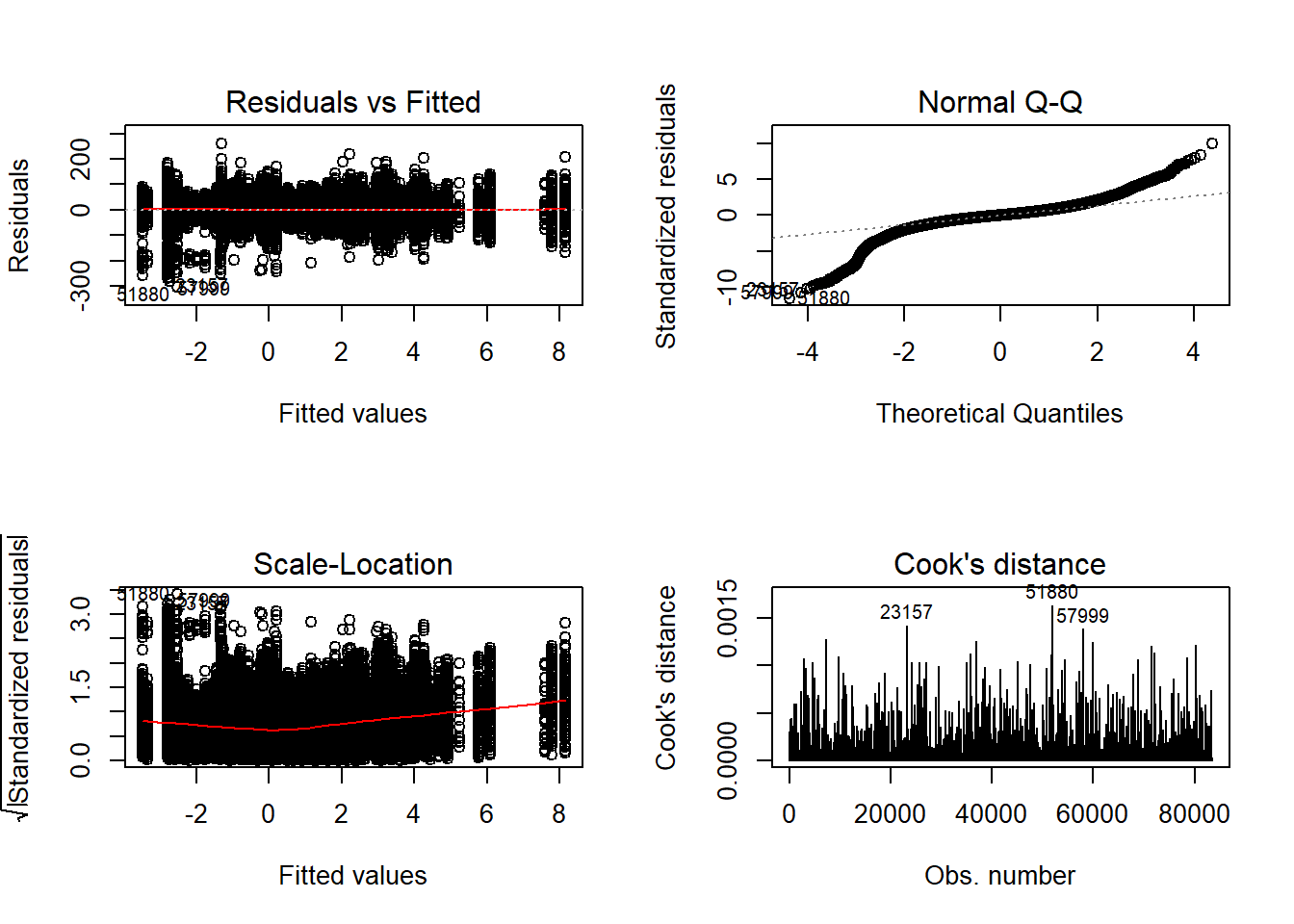


 Shapiro-Wilks Test of Normality of Residuals:

    Shapiro-Wilk normality test

data:  res
W = 0.9, p-value <2e-16


 K-S Test for Normality of Residuals:

    One-sample Kolmogorov-Smirnov test

data:  aov.out$residuals
D = 0.4, p-value <2e-16
alternative hypothesis: two-sided

`stat_bin()` using `bins = 30`. Pick better value with `binwidth`.

Warning: Removed 626 rows containing non-finite values (stat_bin).

Warning: Removed 3 rows containing missing values (geom_bar).

`stat_bin()` using `bins = 30`. Pick better value with `binwidth`.

Warning: Removed 626 rows containing non-finite values (stat_bin).

Warning: Removed 4 rows containing missing values (geom_bar).

`stat_bin()` using `bins = 30`. Pick better value with `binwidth`.

Warning: Removed 626 rows containing non-finite values (stat_bin).

Warning: Removed 3 rows containing missing values (geom_bar).

`stat_bin()` using `bins = 30`. Pick better value with `binwidth`.

Warning: Removed 626 rows containing non-finite values (stat_bin).

Warning: Removed 2 rows containing missing values (geom_bar).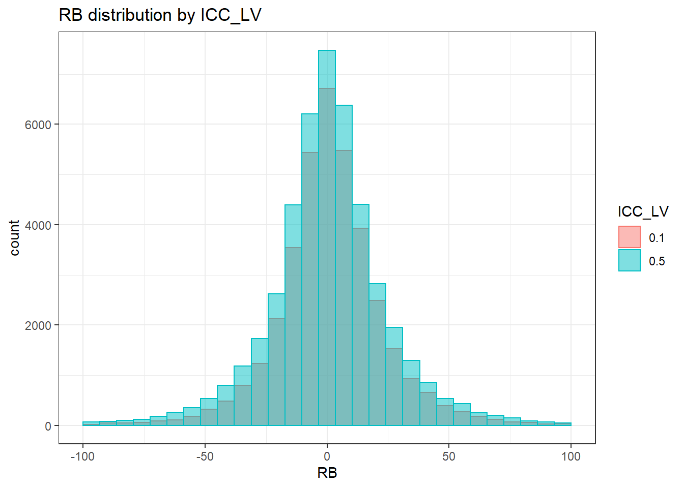

`stat_bin()` using `bins = 30`. Pick better value with `binwidth`.

Warning: Removed 626 rows containing non-finite values (stat_bin).

Warning: Removed 3 rows containing missing values (geom_bar).


 ============================= 

 Tests of Homogeneity of Variance

 
 Levenes Test:  N1 
 
 
Levene's Test for Homogeneity of Variance (center = "mean")
         Df F value Pr(>F)    
group     2    5540 <2e-16 ***
      83507                   
---
Signif. codes:  0 '***' 0.001 '**' 0.01 '*' 0.05 '.' 0.1 ' ' 1

 
 Levenes Test:  N2 
 
 
Levene's Test for Homogeneity of Variance (center = "mean")
         Df F value Pr(>F)    
group     3    3105 <2e-16 ***
      83506                   
---
Signif. codes:  0 '***' 0.001 '**' 0.01 '*' 0.05 '.' 0.1 ' ' 1

 
 Levenes Test:  ICC_OV 
 
 
Levene's Test for Homogeneity of Variance (center = "mean")
         Df F value Pr(>F)    
group     2     492 <2e-16 ***
      83507                   
---
Signif. codes:  0 '***' 0.001 '**' 0.01 '*' 0.05 '.' 0.1 ' ' 1

 
 Levenes Test:  ICC_LV 
 
 
Levene's Test for Homogeneity of Variance (center = "mean")
         Df F value Pr(>F)    
group     1     353 <2e-16 ***
      83508                   
---
Signif. codes:  0 '***' 0.001 '**' 0.01 '*' 0.05 '.' 0.1 ' ' 1

 
 Levenes Test:  Estimator 
 
 
Levene's Test for Homogeneity of Variance (center = "mean")
         Df F value  Pr(>F)    
group     2    26.4 3.3e-12 ***
      83507                    
---
Signif. codes:  0 '***' 0.001 '**' 0.01 '*' 0.05 '.' 0.1 ' ' 1

# was bad... Remove extreme outliers
quantile(sdat$RB, c(0.001, 0.01, 0.99, 0.999))

  0.1%     1%    99%  99.9% 
-191.4  -73.6   71.9  126.4

# remove RB>100
sdat <- filter(sdat, RB <= 100)
boxplot(sdat$RB)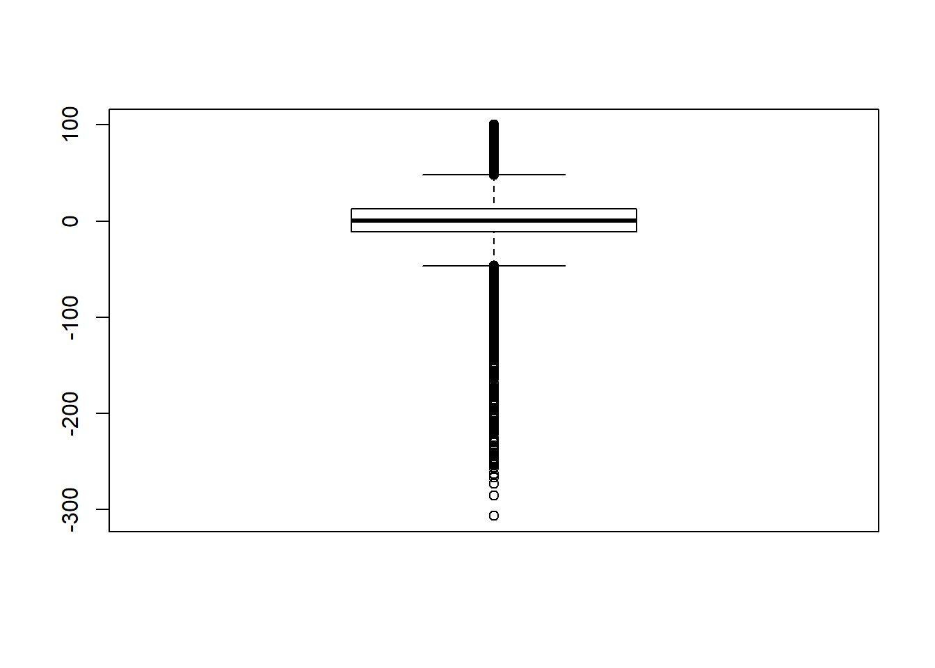

# rerun
## Check assumptions
anova_assumptions_check(
  sdat, 'RB', factors = flist,
  model = as.formula('RB ~ N1 + N2 + ICC_OV + ICC_LV + Estimator + N1:N2 + N1:ICC_OV + N1:ICC_LV + N1:Estimator + N2:ICC_OV + N2:ICC_LV + N2:Estimator + ICC_OV:ICC_LV +  ICC_OV:Estimator  + ICC_LV:Estimator'))


 ============================= 

 Tests and Plots of Normality: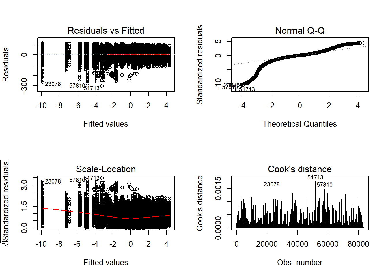


 Shapiro-Wilks Test of Normality of Residuals:

    Shapiro-Wilk normality test

data:  res
W = 0.9, p-value <2e-16


 K-S Test for Normality of Residuals:

    One-sample Kolmogorov-Smirnov test

data:  aov.out$residuals
D = 0.4, p-value <2e-16
alternative hypothesis: two-sided

`stat_bin()` using `bins = 30`. Pick better value with `binwidth`.

Warning: Removed 351 rows containing non-finite values (stat_bin).

Warning: Removed 3 rows containing missing values (geom_bar).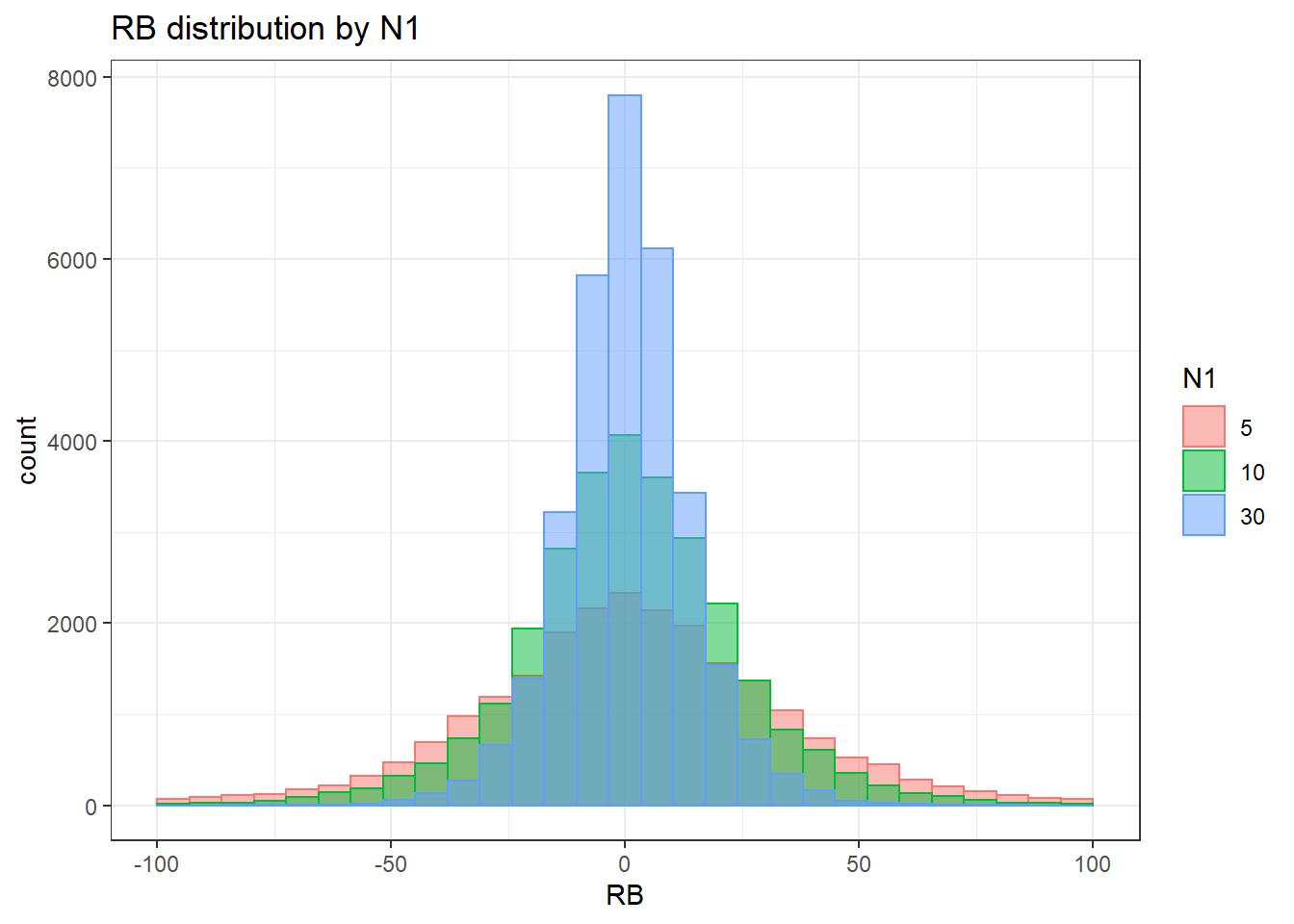

`stat_bin()` using `bins = 30`. Pick better value with `binwidth`.

Warning: Removed 351 rows containing non-finite values (stat_bin).

Warning: Removed 4 rows containing missing values (geom_bar).

`stat_bin()` using `bins = 30`. Pick better value with `binwidth`.

Warning: Removed 351 rows containing non-finite values (stat_bin).

Warning: Removed 3 rows containing missing values (geom_bar).

`stat_bin()` using `bins = 30`. Pick better value with `binwidth`.

Warning: Removed 351 rows containing non-finite values (stat_bin).

Warning: Removed 2 rows containing missing values (geom_bar).

`stat_bin()` using `bins = 30`. Pick better value with `binwidth`.

Warning: Removed 351 rows containing non-finite values (stat_bin).

Warning: Removed 3 rows containing missing values (geom_bar).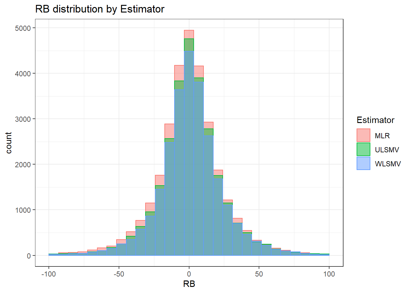


 ============================= 

 Tests of Homogeneity of Variance

 
 Levenes Test:  N1 
 
 
Levene's Test for Homogeneity of Variance (center = "mean")
         Df F value Pr(>F)    
group     2    5347 <2e-16 ***
      83232                   
---
Signif. codes:  0 '***' 0.001 '**' 0.01 '*' 0.05 '.' 0.1 ' ' 1

 
 Levenes Test:  N2 
 
 
Levene's Test for Homogeneity of Variance (center = "mean")
         Df F value Pr(>F)    
group     3    2970 <2e-16 ***
      83231                   
---
Signif. codes:  0 '***' 0.001 '**' 0.01 '*' 0.05 '.' 0.1 ' ' 1

 
 Levenes Test:  ICC_OV 
 
 
Levene's Test for Homogeneity of Variance (center = "mean")
         Df F value Pr(>F)    
group     2     465 <2e-16 ***
      83232                   
---
Signif. codes:  0 '***' 0.001 '**' 0.01 '*' 0.05 '.' 0.1 ' ' 1

 
 Levenes Test:  ICC_LV 
 
 
Levene's Test for Homogeneity of Variance (center = "mean")
         Df F value Pr(>F)    
group     1     379 <2e-16 ***
      83233                   
---
Signif. codes:  0 '***' 0.001 '**' 0.01 '*' 0.05 '.' 0.1 ' ' 1

 
 Levenes Test:  Estimator 
 
 
Levene's Test for Homogeneity of Variance (center = "mean")
         Df F value  Pr(>F)    
group     2    27.1 1.6e-12 ***
      83232                    
---
Signif. codes:  0 '***' 0.001 '**' 0.01 '*' 0.05 '.' 0.1 ' ' 1

ANOVA Results

model = as.formula('RB ~ N1 + N2 + ICC_OV + ICC_LV + Estimator + N1:N2 + N1:ICC_OV + N1:ICC_LV + N1:Estimator + N2:ICC_OV + N2:ICC_LV + N2:Estimator + ICC_OV:ICC_LV +  ICC_OV:Estimator  + ICC_LV:Estimator')

fit <- aov(model, data = sdat)
fit.out <- summary(fit)
fit.out

                    Df   Sum Sq Mean Sq F value  Pr(>F)    
N1                   2    12098    6049    9.58 6.9e-05 ***
N2                   3    12985    4328    6.86 0.00013 ***
ICC_OV               2    13539    6770   10.72 2.2e-05 ***
ICC_LV               1    38331   38331   60.72 6.7e-15 ***
Estimator            2    32169   16084   25.48 8.7e-12 ***
N1:N2                6    72784   12131   19.22 < 2e-16 ***
N1:ICC_OV            4    11146    2786    4.41 0.00144 ** 
N1:ICC_LV            2    23091   11546   18.29 1.1e-08 ***
N1:Estimator         4     8807    2202    3.49 0.00746 ** 
N2:ICC_OV            6     3309     551    0.87 0.51327    
N2:ICC_LV            3     2618     873    1.38 0.24610    
N2:Estimator         6    16206    2701    4.28 0.00026 ***
ICC_OV:ICC_LV        2     3388    1694    2.68 0.06832 .  
ICC_OV:Estimator     4    21821    5455    8.64 5.7e-07 ***
ICC_LV:Estimator     2    21537   10768   17.06 3.9e-08 ***
Residuals        83185 52514022     631                    
---
Signif. codes:  0 '***' 0.001 '**' 0.01 '*' 0.05 '.' 0.1 ' ' 1

resultsList[["Level1-FactorCovariance"]] <- cbind(omega2(fit.out), p_omega2(fit.out))
resultsList[["Level1-FactorCovariance"]]

                 omega^2 partial-omega^2
N1                0.0002          0.0002
N2                0.0002          0.0002
ICC_OV            0.0002          0.0002
ICC_LV            0.0007          0.0007
Estimator         0.0006          0.0006
N1:N2             0.0013          0.0013
N1:ICC_OV         0.0002          0.0002
N1:ICC_LV         0.0004          0.0004
N1:Estimator      0.0001          0.0001
N2:ICC_OV         0.0000          0.0000
N2:ICC_LV         0.0000          0.0000
N2:Estimator      0.0002          0.0002
ICC_OV:ICC_LV     0.0000          0.0000
ICC_OV:Estimator  0.0004          0.0004
ICC_LV:Estimator  0.0004          0.0004

Level-2 factor (co)variances

Assumption Checking

sdat <- filter(long_results, Parameter %like% "psiB")

sdat <- sdat %>%
  group_by(Replication, N1, N2, ICC_OV, ICC_LV, Estimator) %>%
  summarise(RB = mean(RB))

# first, look at summary of RB Estimates
boxplot(sdat$RB)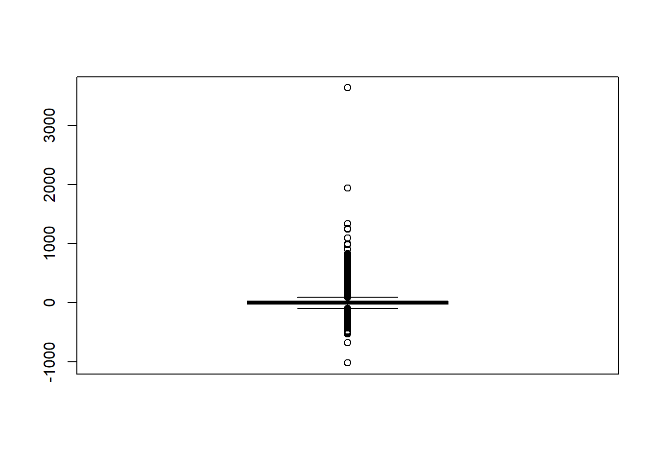

## model factors...
flist <- c('N1', 'N2', 'ICC_OV', 'ICC_LV', 'Estimator')
## Check assumptions
anova_assumptions_check(
  sdat, 'RB', factors = flist,
  model = as.formula('RB ~ N1 + N2 + ICC_OV + ICC_LV + Estimator + N1:N2 + N1:ICC_OV + N1:ICC_LV + N1:Estimator + N2:ICC_OV + N2:ICC_LV + N2:Estimator + ICC_OV:ICC_LV +  ICC_OV:Estimator  + ICC_LV:Estimator'))


 ============================= 

 Tests and Plots of Normality: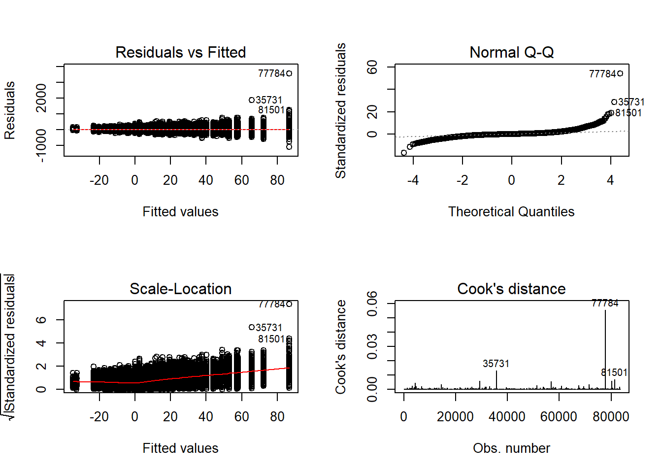


 Shapiro-Wilks Test of Normality of Residuals:

    Shapiro-Wilk normality test

data:  res
W = 0.9, p-value <2e-16


 K-S Test for Normality of Residuals:

    One-sample Kolmogorov-Smirnov test

data:  aov.out$residuals
D = 0.5, p-value <2e-16
alternative hypothesis: two-sided

`stat_bin()` using `bins = 30`. Pick better value with `binwidth`.

Warning: Removed 6886 rows containing non-finite values (stat_bin).

Warning: Removed 3 rows containing missing values (geom_bar).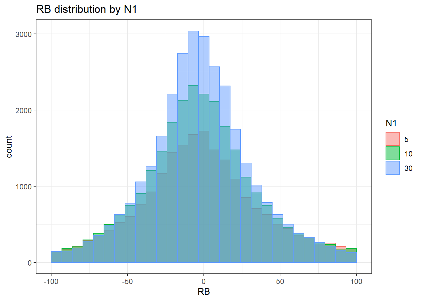

`stat_bin()` using `bins = 30`. Pick better value with `binwidth`.

Warning: Removed 6886 rows containing non-finite values (stat_bin).

Warning: Removed 4 rows containing missing values (geom_bar).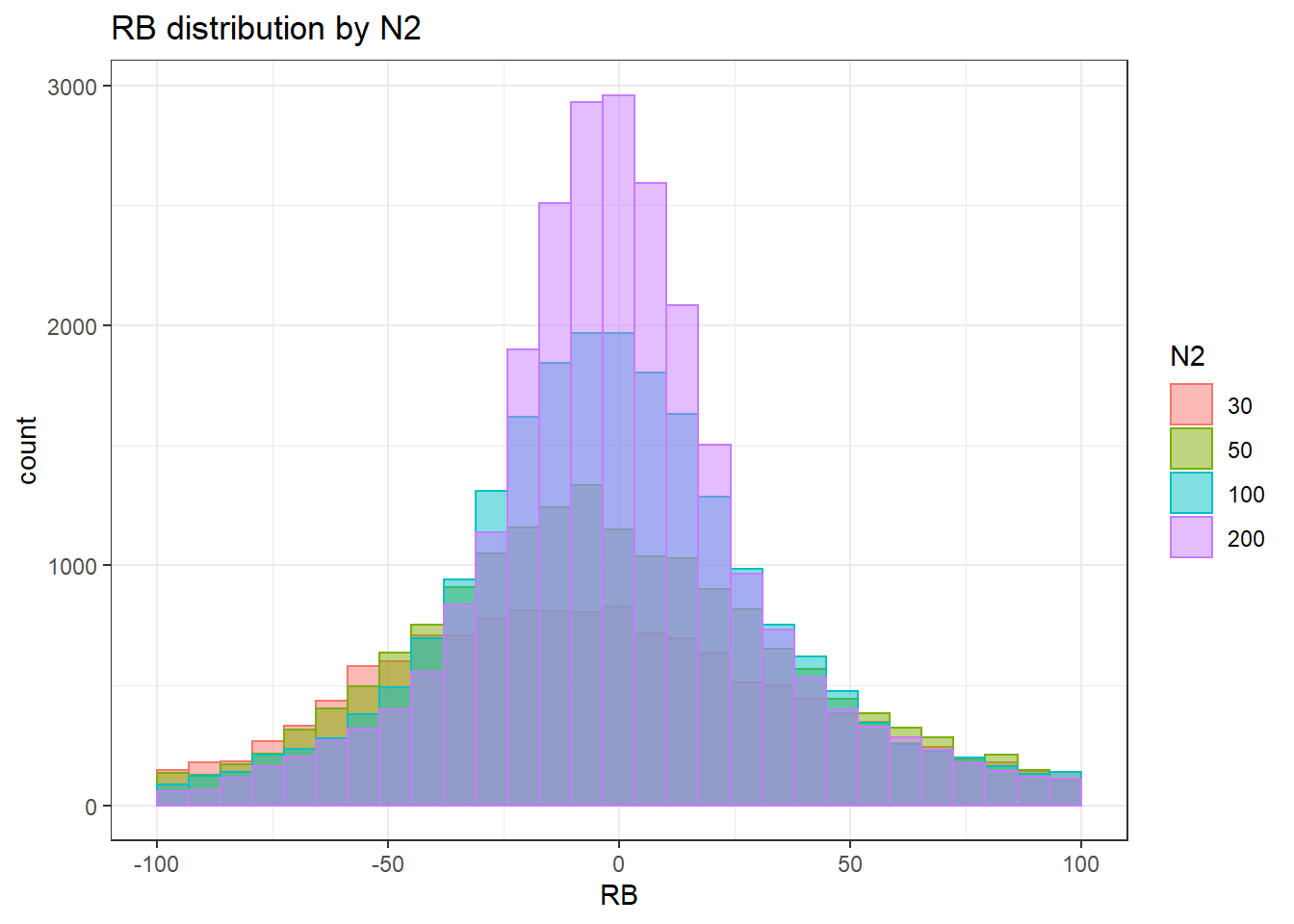

`stat_bin()` using `bins = 30`. Pick better value with `binwidth`.

Warning: Removed 6886 rows containing non-finite values (stat_bin).

Warning: Removed 3 rows containing missing values (geom_bar).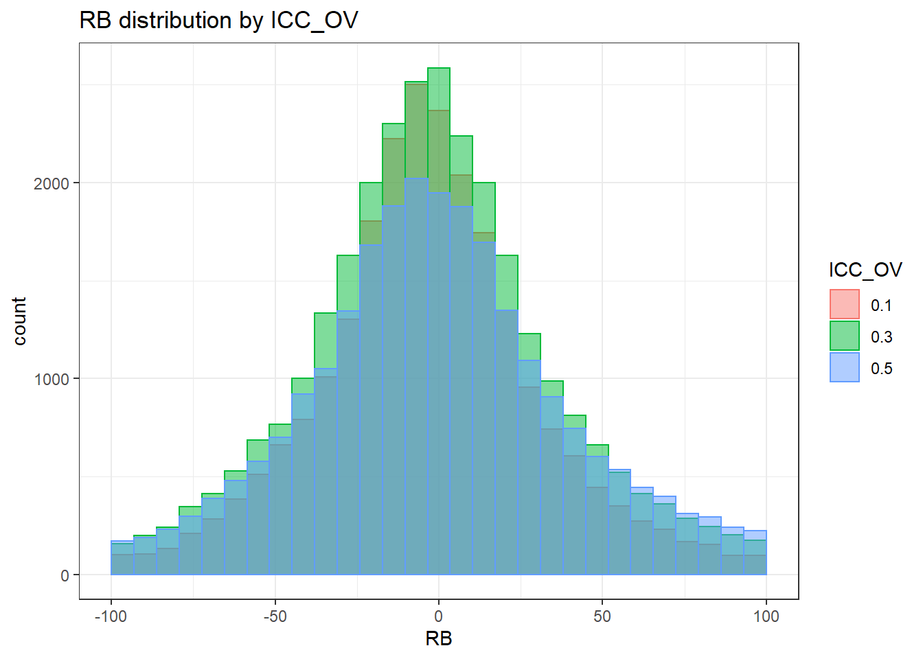

`stat_bin()` using `bins = 30`. Pick better value with `binwidth`.

Warning: Removed 6886 rows containing non-finite values (stat_bin).

Warning: Removed 2 rows containing missing values (geom_bar).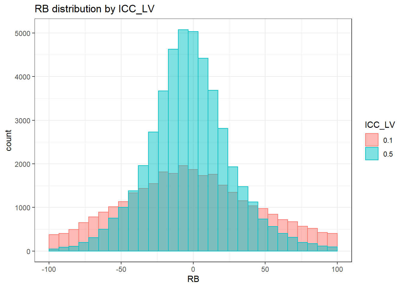

`stat_bin()` using `bins = 30`. Pick better value with `binwidth`.

Warning: Removed 6886 rows containing non-finite values (stat_bin).

Warning: Removed 3 rows containing missing values (geom_bar).


 ============================= 

 Tests of Homogeneity of Variance

 
 Levenes Test:  N1 
 
 
Levene's Test for Homogeneity of Variance (center = "mean")
         Df F value Pr(>F)    
group     2     786 <2e-16 ***
      83507                   
---
Signif. codes:  0 '***' 0.001 '**' 0.01 '*' 0.05 '.' 0.1 ' ' 1

 
 Levenes Test:  N2 
 
 
Levene's Test for Homogeneity of Variance (center = "mean")
         Df F value Pr(>F)    
group     3    2028 <2e-16 ***
      83506                   
---
Signif. codes:  0 '***' 0.001 '**' 0.01 '*' 0.05 '.' 0.1 ' ' 1

 
 Levenes Test:  ICC_OV 
 
 
Levene's Test for Homogeneity of Variance (center = "mean")
         Df F value Pr(>F)    
group     2    1269 <2e-16 ***
      83507                   
---
Signif. codes:  0 '***' 0.001 '**' 0.01 '*' 0.05 '.' 0.1 ' ' 1

 
 Levenes Test:  ICC_LV 
 
 
Levene's Test for Homogeneity of Variance (center = "mean")
         Df F value Pr(>F)    
group     1   11718 <2e-16 ***
      83508                   
---
Signif. codes:  0 '***' 0.001 '**' 0.01 '*' 0.05 '.' 0.1 ' ' 1

 
 Levenes Test:  Estimator 
 
 
Levene's Test for Homogeneity of Variance (center = "mean")
         Df F value Pr(>F)    
group     2     125 <2e-16 ***
      83507                   
---
Signif. codes:  0 '***' 0.001 '**' 0.01 '*' 0.05 '.' 0.1 ' ' 1

# was bad... Remove extreme outliers
quantile(sdat$RB, c(0.001, 0.01, 0.99, 0.999))

 0.1%    1%   99% 99.9% 
 -281  -152   233   507

# remove RB>100
sdat <- filter(sdat, RB <= 100)
boxplot(sdat$RB)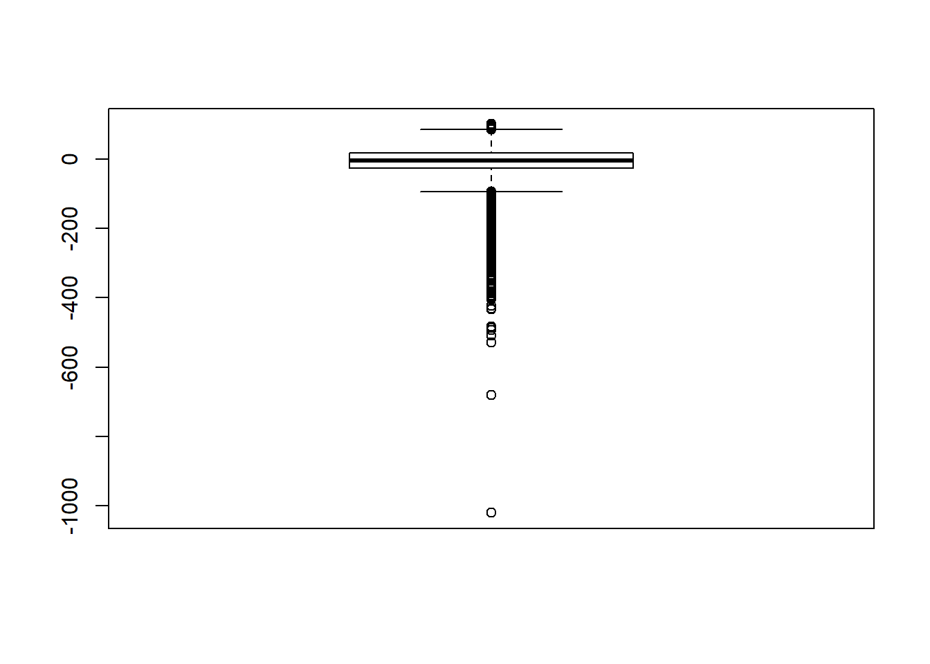

# rerun
## Check assumptions
anova_assumptions_check(
  sdat, 'RB', factors = flist,
  model = as.formula('RB ~ N1 + N2 + ICC_OV + ICC_LV + Estimator + N1:N2 + N1:ICC_OV + N1:ICC_LV + N1:Estimator + N2:ICC_OV + N2:ICC_LV + N2:Estimator + ICC_OV:ICC_LV +  ICC_OV:Estimator  + ICC_LV:Estimator'))


 ============================= 

 Tests and Plots of Normality: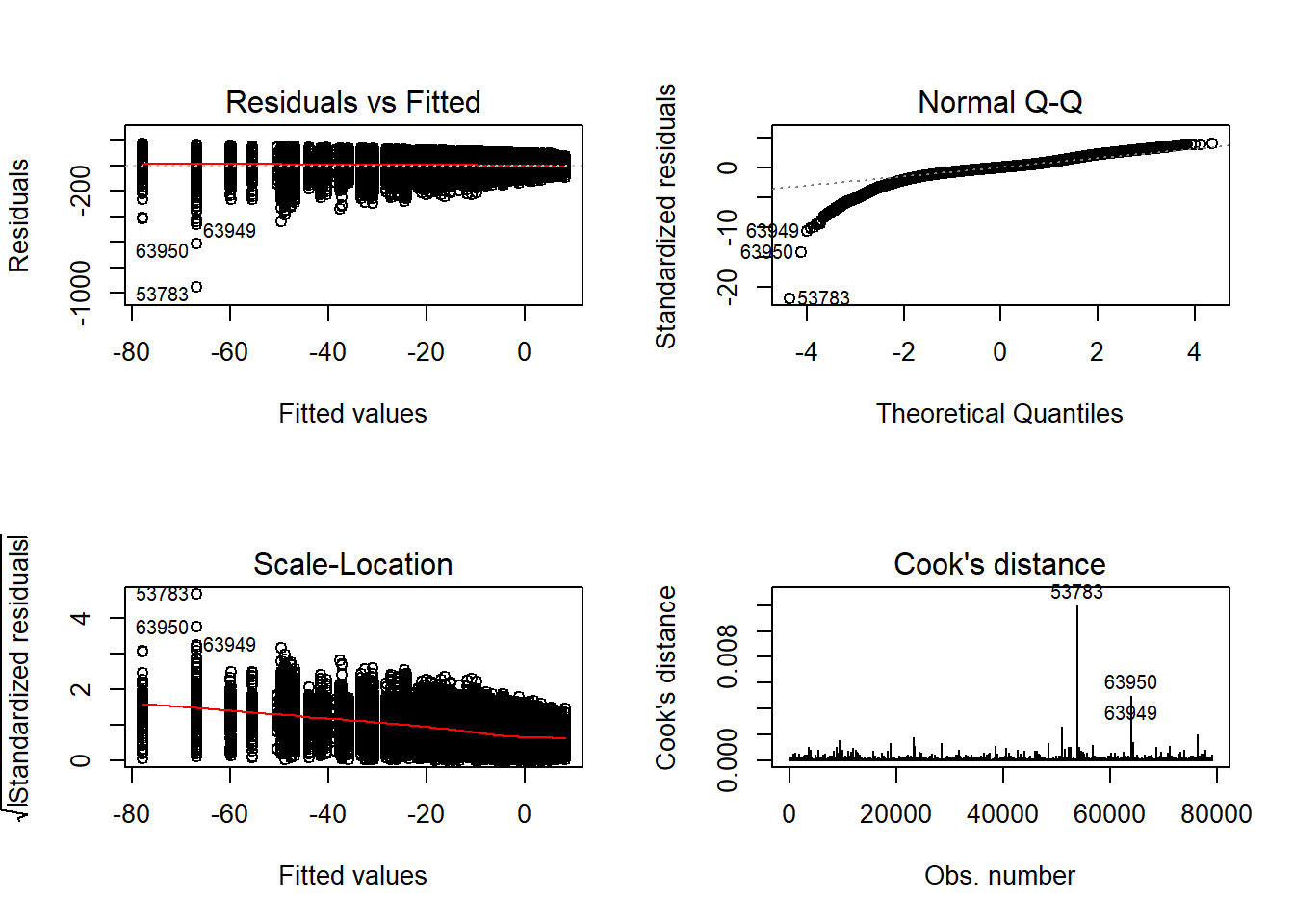


 Shapiro-Wilks Test of Normality of Residuals:

    Shapiro-Wilk normality test

data:  res
W = 1, p-value <2e-16


 K-S Test for Normality of Residuals:

    One-sample Kolmogorov-Smirnov test

data:  aov.out$residuals
D = 0.5, p-value <2e-16
alternative hypothesis: two-sided

`stat_bin()` using `bins = 30`. Pick better value with `binwidth`.

Warning: Removed 2414 rows containing non-finite values (stat_bin).

Warning: Removed 3 rows containing missing values (geom_bar).

`stat_bin()` using `bins = 30`. Pick better value with `binwidth`.

Warning: Removed 2414 rows containing non-finite values (stat_bin).

Warning: Removed 4 rows containing missing values (geom_bar).

`stat_bin()` using `bins = 30`. Pick better value with `binwidth`.

Warning: Removed 2414 rows containing non-finite values (stat_bin).

Warning: Removed 3 rows containing missing values (geom_bar).

`stat_bin()` using `bins = 30`. Pick better value with `binwidth`.

Warning: Removed 2414 rows containing non-finite values (stat_bin).

Warning: Removed 2 rows containing missing values (geom_bar).

`stat_bin()` using `bins = 30`. Pick better value with `binwidth`.

Warning: Removed 2414 rows containing non-finite values (stat_bin).

Warning: Removed 3 rows containing missing values (geom_bar).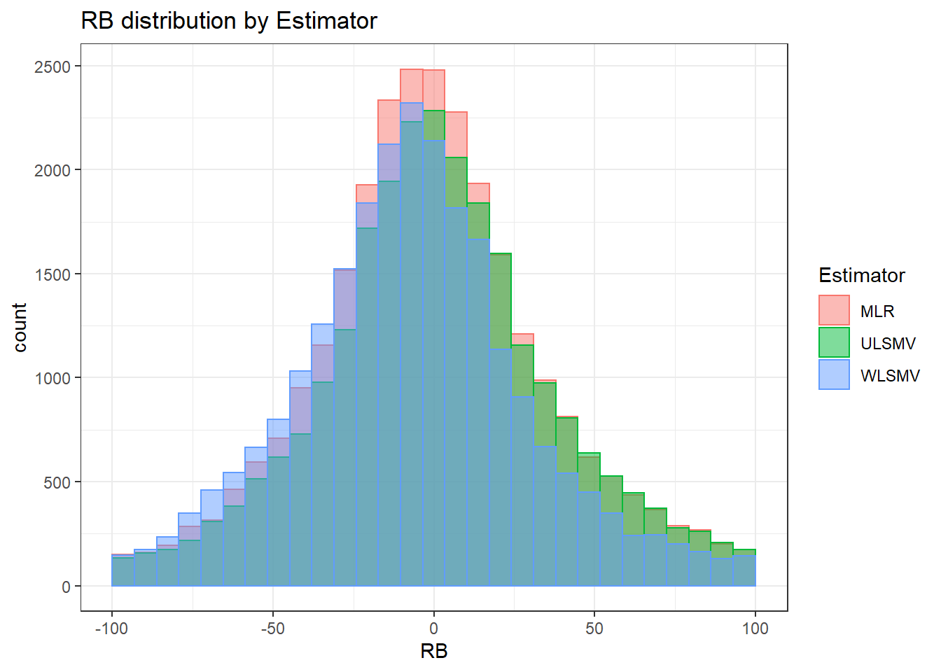


 ============================= 

 Tests of Homogeneity of Variance

 
 Levenes Test:  N1 
 
 
Levene's Test for Homogeneity of Variance (center = "mean")
         Df F value Pr(>F)    
group     2     489 <2e-16 ***
      79035                   
---
Signif. codes:  0 '***' 0.001 '**' 0.01 '*' 0.05 '.' 0.1 ' ' 1

 
 Levenes Test:  N2 
 
 
Levene's Test for Homogeneity of Variance (center = "mean")
         Df F value Pr(>F)    
group     3    1476 <2e-16 ***
      79034                   
---
Signif. codes:  0 '***' 0.001 '**' 0.01 '*' 0.05 '.' 0.1 ' ' 1

 
 Levenes Test:  ICC_OV 
 
 
Levene's Test for Homogeneity of Variance (center = "mean")
         Df F value Pr(>F)    
group     2     673 <2e-16 ***
      79035                   
---
Signif. codes:  0 '***' 0.001 '**' 0.01 '*' 0.05 '.' 0.1 ' ' 1

 
 Levenes Test:  ICC_LV 
 
 
Levene's Test for Homogeneity of Variance (center = "mean")
         Df F value Pr(>F)    
group     1   10946 <2e-16 ***
      79036                   
---
Signif. codes:  0 '***' 0.001 '**' 0.01 '*' 0.05 '.' 0.1 ' ' 1

 
 Levenes Test:  Estimator 
 
 
Levene's Test for Homogeneity of Variance (center = "mean")
         Df F value  Pr(>F)    
group     2    8.14 0.00029 ***
      79035                    
---
Signif. codes:  0 '***' 0.001 '**' 0.01 '*' 0.05 '.' 0.1 ' ' 1

ANOVA Results

model = as.formula('RB ~ N1 + N2 + ICC_OV + ICC_LV + Estimator + N1:N2 + N1:ICC_OV + N1:ICC_LV + N1:Estimator + N2:ICC_OV + N2:ICC_LV + N2:Estimator + ICC_OV:ICC_LV +  ICC_OV:Estimator  + ICC_LV:Estimator')

fit <- aov(model, data = sdat)
fit.out <- summary(fit)
fit.out

                    Df   Sum Sq Mean Sq F value  Pr(>F)    
N1                   2 2.71e+05  135524   71.34 < 2e-16 ***
N2                   3 2.31e+06  770291  405.51 < 2e-16 ***
ICC_OV               2 9.59e+04   47937   25.24 1.1e-11 ***
ICC_LV               1 2.99e+06 2991922 1575.05 < 2e-16 ***
Estimator            2 7.70e+05  384823  202.58 < 2e-16 ***
N1:N2                6 2.91e+05   48542   25.55 < 2e-16 ***
N1:ICC_OV            4 1.76e+04    4394    2.31   0.055 .  
N1:ICC_LV            2 5.94e+05  296985  156.34 < 2e-16 ***
N1:Estimator         4 1.74e+03     434    0.23   0.923    
N2:ICC_OV            6 7.92e+04   13196    6.95 2.1e-07 ***
N2:ICC_LV            3 2.38e+06  792029  416.95 < 2e-16 ***
N2:Estimator         6 1.97e+05   32868   17.30 < 2e-16 ***
ICC_OV:ICC_LV        2 8.56e+05  428080  225.36 < 2e-16 ***
ICC_OV:Estimator     4 2.17e+04    5430    2.86   0.022 *  
ICC_LV:Estimator     2 1.10e+05   54753   28.82 3.1e-13 ***
Residuals        78988 1.50e+08    1900                    
---
Signif. codes:  0 '***' 0.001 '**' 0.01 '*' 0.05 '.' 0.1 ' ' 1

resultsList[["Level2-FactorCovariance"]] <- cbind(omega2(fit.out), p_omega2(fit.out))
resultsList[["Level2-FactorCovariance"]]

                 omega^2 partial-omega^2
N1                0.0017          0.0018
N2                0.0143          0.0151
ICC_OV            0.0006          0.0006
ICC_LV            0.0186          0.0195
Estimator         0.0048          0.0051
N1:N2             0.0017          0.0019
N1:ICC_OV         0.0001          0.0001
N1:ICC_LV         0.0037          0.0039
N1:Estimator      0.0000          0.0000
N2:ICC_OV         0.0004          0.0005
N2:ICC_LV         0.0147          0.0155
N2:Estimator      0.0012          0.0012
ICC_OV:ICC_LV     0.0053          0.0056
ICC_OV:Estimator  0.0001          0.0001
ICC_LV:Estimator  0.0007          0.0007

Level-2 item residual variances

Assumption Checking

sdat <- filter(long_results, Parameter %like% "thetaB")

sdat <- sdat %>%
  group_by(Replication, N1, N2, ICC_OV, ICC_LV, Estimator) %>%
  summarise(RB = mean(RB))

# first, look at summary of RB Estimates
boxplot(sdat$RB)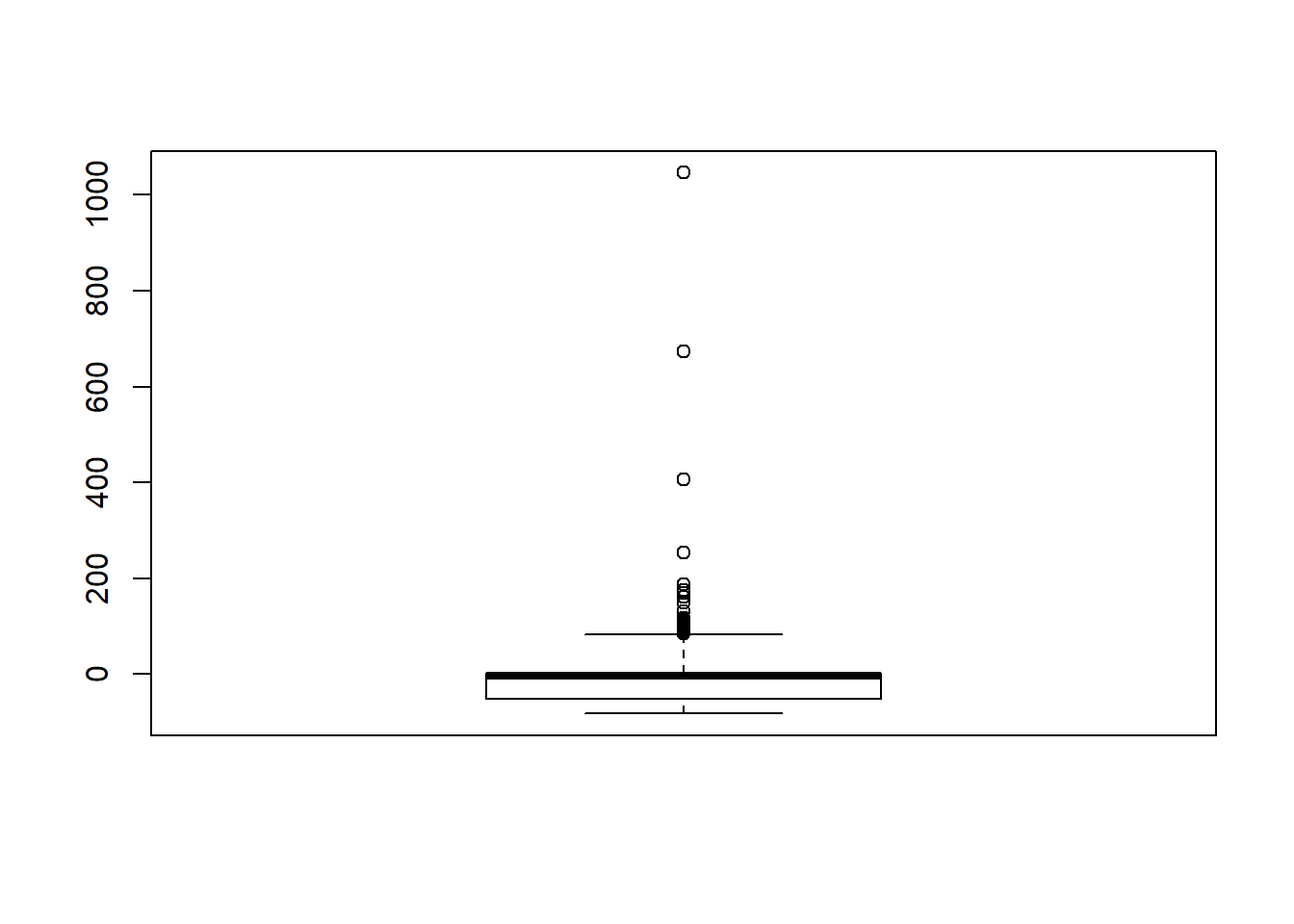

## model factors...
flist <- c('N1', 'N2', 'ICC_OV', 'ICC_LV', 'Estimator')
## Check assumptions
anova_assumptions_check(
  sdat, 'RB', factors = flist,
  model = as.formula('RB ~ N1 + N2 + ICC_OV + ICC_LV + Estimator + N1:N2 + N1:ICC_OV + N1:ICC_LV + N1:Estimator + N2:ICC_OV + N2:ICC_LV + N2:Estimator + ICC_OV:ICC_LV +  ICC_OV:Estimator  + ICC_LV:Estimator'))


 ============================= 

 Tests and Plots of Normality: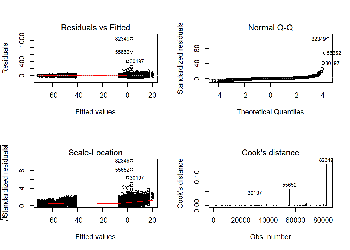


 Shapiro-Wilks Test of Normality of Residuals:

    Shapiro-Wilk normality test

data:  res
W = 0.7, p-value <2e-16


 K-S Test for Normality of Residuals:

    One-sample Kolmogorov-Smirnov test

data:  aov.out$residuals
D = 0.3, p-value <2e-16
alternative hypothesis: two-sided

`stat_bin()` using `bins = 30`. Pick better value with `binwidth`.

Warning: Removed 16 rows containing non-finite values (stat_bin).

Warning: Removed 3 rows containing missing values (geom_bar).

`stat_bin()` using `bins = 30`. Pick better value with `binwidth`.

Warning: Removed 16 rows containing non-finite values (stat_bin).

Warning: Removed 4 rows containing missing values (geom_bar).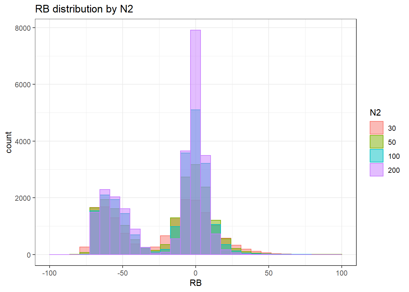

`stat_bin()` using `bins = 30`. Pick better value with `binwidth`.

Warning: Removed 16 rows containing non-finite values (stat_bin).

Warning: Removed 3 rows containing missing values (geom_bar).

`stat_bin()` using `bins = 30`. Pick better value with `binwidth`.

Warning: Removed 16 rows containing non-finite values (stat_bin).

Warning: Removed 2 rows containing missing values (geom_bar).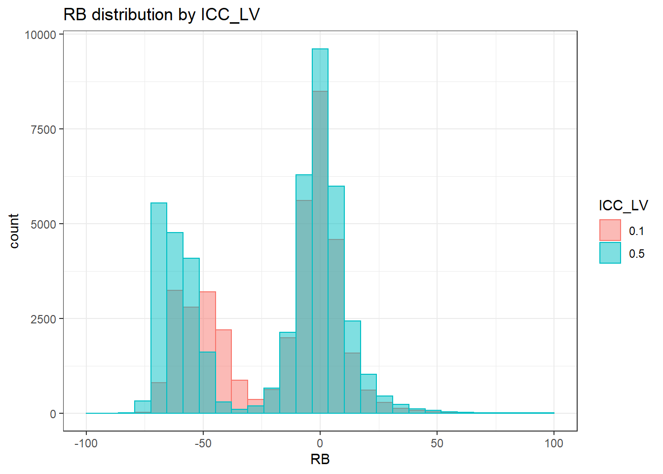

`stat_bin()` using `bins = 30`. Pick better value with `binwidth`.

Warning: Removed 16 rows containing non-finite values (stat_bin).

Warning: Removed 3 rows containing missing values (geom_bar).


 ============================= 

 Tests of Homogeneity of Variance

 
 Levenes Test:  N1 
 
 
Levene's Test for Homogeneity of Variance (center = "mean")
         Df F value Pr(>F)    
group     2     535 <2e-16 ***
      83507                   
---
Signif. codes:  0 '***' 0.001 '**' 0.01 '*' 0.05 '.' 0.1 ' ' 1

 
 Levenes Test:  N2 
 
 
Levene's Test for Homogeneity of Variance (center = "mean")
         Df F value Pr(>F)    
group     3     290 <2e-16 ***
      83506                   
---
Signif. codes:  0 '***' 0.001 '**' 0.01 '*' 0.05 '.' 0.1 ' ' 1

 
 Levenes Test:  ICC_OV 
 
 
Levene's Test for Homogeneity of Variance (center = "mean")
         Df F value Pr(>F)    
group     2    1265 <2e-16 ***
      83507                   
---
Signif. codes:  0 '***' 0.001 '**' 0.01 '*' 0.05 '.' 0.1 ' ' 1

 
 Levenes Test:  ICC_LV 
 
 
Levene's Test for Homogeneity of Variance (center = "mean")
         Df F value Pr(>F)    
group     1    2710 <2e-16 ***
      83508                   
---
Signif. codes:  0 '***' 0.001 '**' 0.01 '*' 0.05 '.' 0.1 ' ' 1

 
 Levenes Test:  Estimator 
 
 
Levene's Test for Homogeneity of Variance (center = "mean")
         Df F value Pr(>F)    
group     2    36.3 <2e-16 ***
      83507                   
---
Signif. codes:  0 '***' 0.001 '**' 0.01 '*' 0.05 '.' 0.1 ' ' 1

# was bad... Remove extreme outliers
quantile(sdat$RB, c(0.001, 0.01, 0.99, 0.999))

 0.1%    1%   99% 99.9% 
-74.7 -70.8  30.4  60.2

# remove RB>100
sdat <- filter(sdat, RB <= 100)
boxplot(sdat$RB)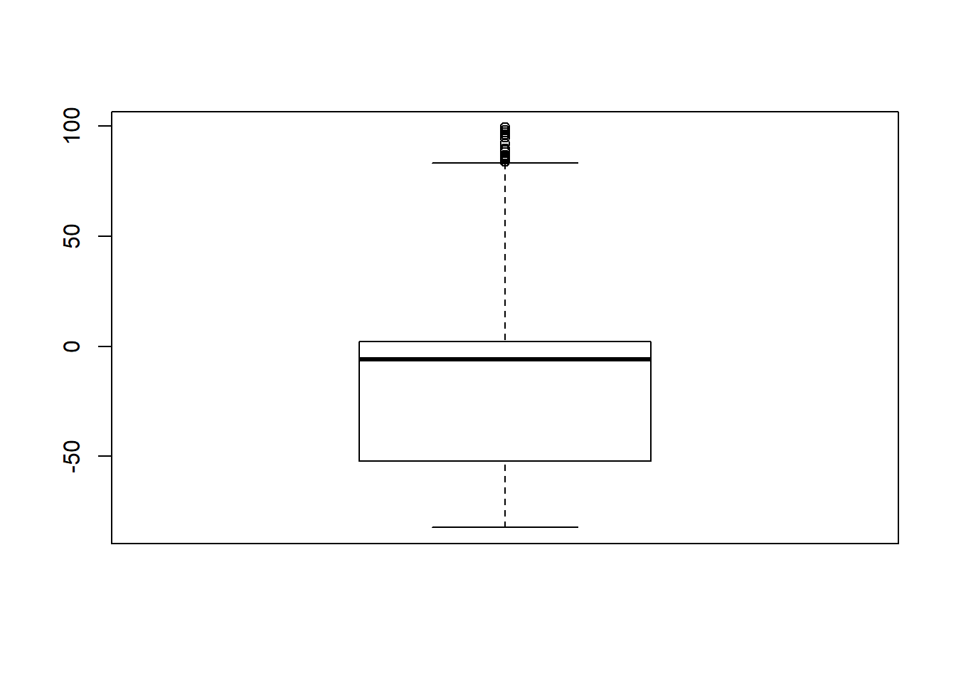

# rerun
## Check assumptions
anova_assumptions_check(
  sdat, 'RB', factors = flist,
  model = as.formula('RB ~ N1 + N2 + ICC_OV + ICC_LV + Estimator + N1:N2 + N1:ICC_OV + N1:ICC_LV + N1:Estimator + N2:ICC_OV + N2:ICC_LV + N2:Estimator + ICC_OV:ICC_LV +  ICC_OV:Estimator  + ICC_LV:Estimator'))


 ============================= 

 Tests and Plots of Normality: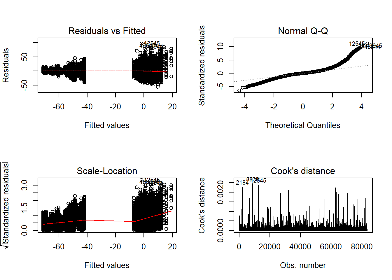


 Shapiro-Wilks Test of Normality of Residuals:

    Shapiro-Wilk normality test

data:  res
W = 0.9, p-value <2e-16


 K-S Test for Normality of Residuals:

    One-sample Kolmogorov-Smirnov test

data:  aov.out$residuals
D = 0.3, p-value <2e-16
alternative hypothesis: two-sided

`stat_bin()` using `bins = 30`. Pick better value with `binwidth`.

Warning: Removed 3 rows containing missing values (geom_bar).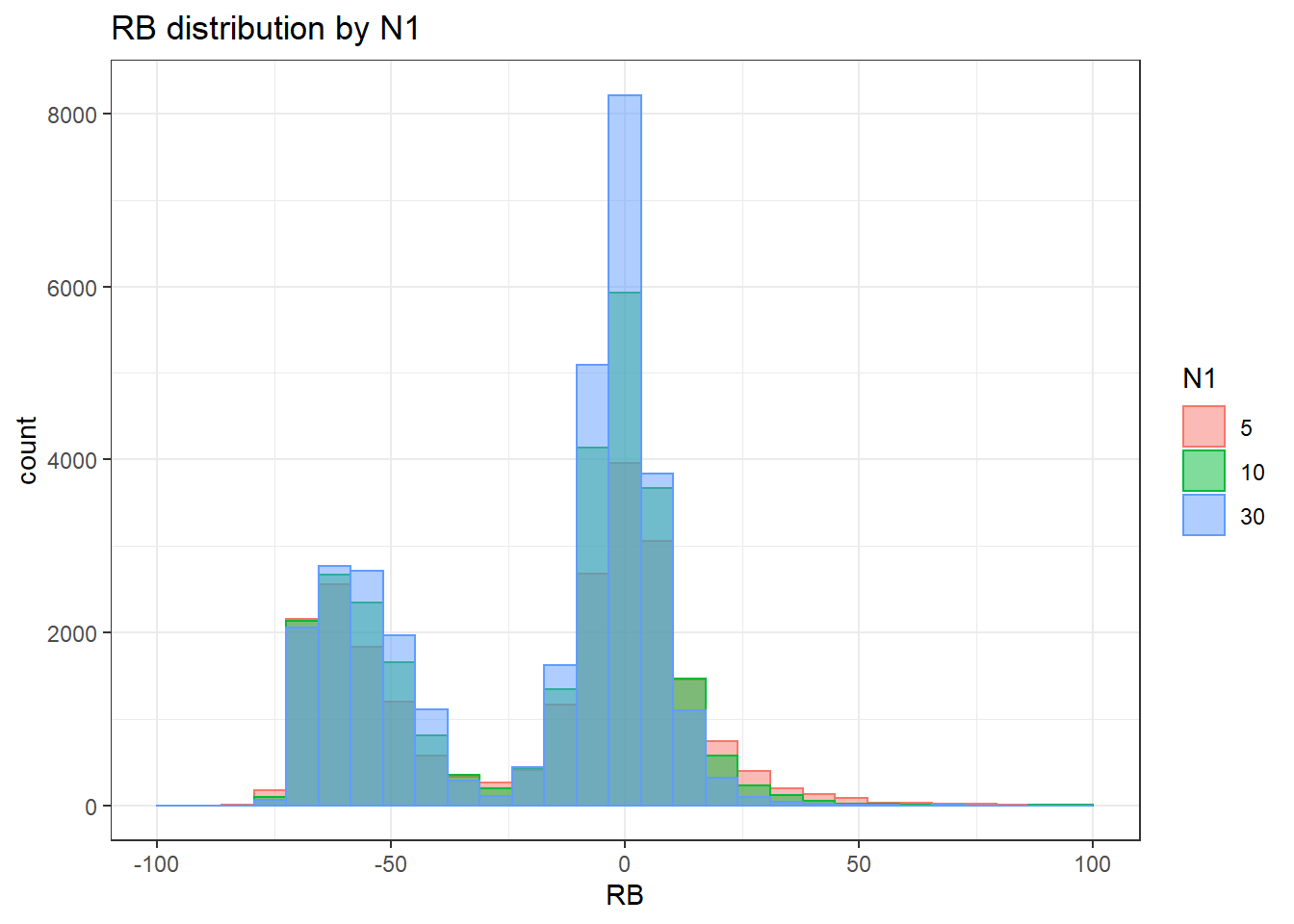

`stat_bin()` using `bins = 30`. Pick better value with `binwidth`.

Warning: Removed 4 rows containing missing values (geom_bar).

`stat_bin()` using `bins = 30`. Pick better value with `binwidth`.

Warning: Removed 3 rows containing missing values (geom_bar).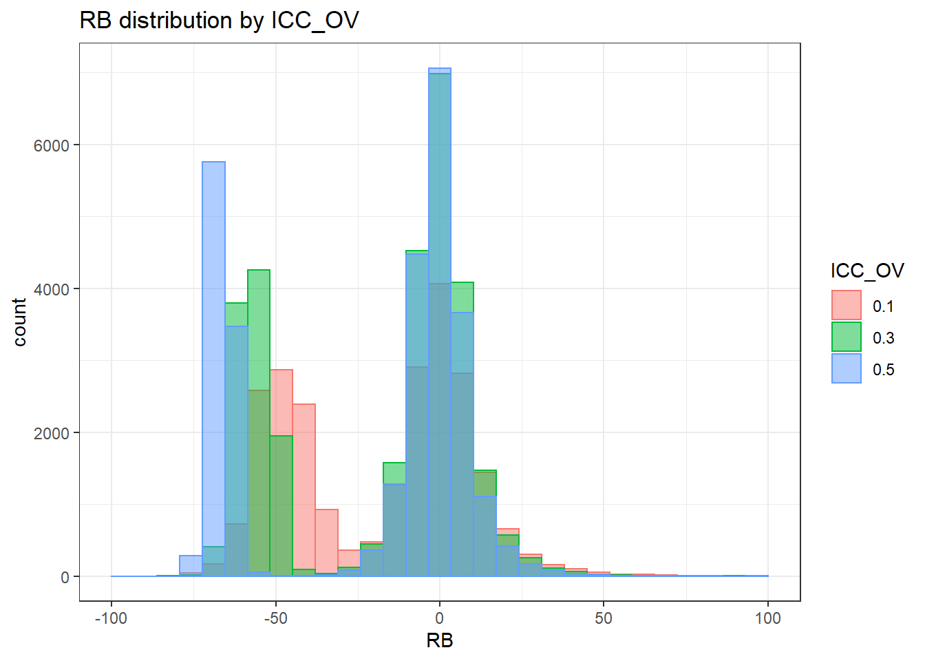

`stat_bin()` using `bins = 30`. Pick better value with `binwidth`.

Warning: Removed 2 rows containing missing values (geom_bar).

`stat_bin()` using `bins = 30`. Pick better value with `binwidth`.

Warning: Removed 3 rows containing missing values (geom_bar).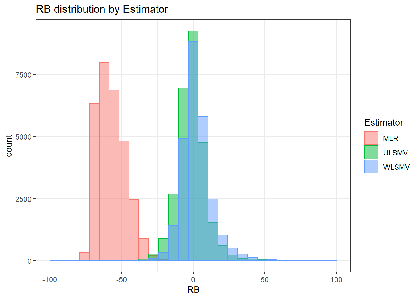


 ============================= 

 Tests of Homogeneity of Variance

 
 Levenes Test:  N1 
 
 
Levene's Test for Homogeneity of Variance (center = "mean")
         Df F value Pr(>F)    
group     2     577 <2e-16 ***
      83491                   
---
Signif. codes:  0 '***' 0.001 '**' 0.01 '*' 0.05 '.' 0.1 ' ' 1

 
 Levenes Test:  N2 
 
 
Levene's Test for Homogeneity of Variance (center = "mean")
         Df F value Pr(>F)    
group     3     304 <2e-16 ***
      83490                   
---
Signif. codes:  0 '***' 0.001 '**' 0.01 '*' 0.05 '.' 0.1 ' ' 1

 
 Levenes Test:  ICC_OV 
 
 
Levene's Test for Homogeneity of Variance (center = "mean")
         Df F value Pr(>F)    
group     2    1439 <2e-16 ***
      83491                   
---
Signif. codes:  0 '***' 0.001 '**' 0.01 '*' 0.05 '.' 0.1 ' ' 1

 
 Levenes Test:  ICC_LV 
 
 
Levene's Test for Homogeneity of Variance (center = "mean")
         Df F value Pr(>F)    
group     1    3097 <2e-16 ***
      83492                   
---
Signif. codes:  0 '***' 0.001 '**' 0.01 '*' 0.05 '.' 0.1 ' ' 1

 
 Levenes Test:  Estimator 
 
 
Levene's Test for Homogeneity of Variance (center = "mean")
         Df F value Pr(>F)    
group     2    83.5 <2e-16 ***
      83491                   
---
Signif. codes:  0 '***' 0.001 '**' 0.01 '*' 0.05 '.' 0.1 ' ' 1

ANOVA Results

model = as.formula('RB ~ N1 + N2 + ICC_OV + ICC_LV + Estimator + N1:N2 + N1:ICC_OV + N1:ICC_LV + N1:Estimator + N2:ICC_OV + N2:ICC_LV + N2:Estimator + ICC_OV:ICC_LV +  ICC_OV:Estimator  + ICC_LV:Estimator')

fit <- aov(model, data = sdat)
fit.out <- summary(fit)
fit.out

                    Df   Sum Sq  Mean Sq  F value Pr(>F)    
N1                   2     1810      905 1.22e+01  5e-06 ***
N2                   3   120963    40321 5.44e+02 <2e-16 ***
ICC_OV               2   221528   110764 1.50e+03 <2e-16 ***
ICC_LV               1   117591   117591 1.59e+03 <2e-16 ***
Estimator            2 64714778 32357389 4.37e+05 <2e-16 ***
N1:N2                6    40179     6697 9.04e+01 <2e-16 ***
N1:ICC_OV            4    21922     5480 7.40e+01 <2e-16 ***
N1:ICC_LV            2      986      493 6.65e+00 0.0013 ** 
N1:Estimator         4   133862    33465 4.52e+02 <2e-16 ***
N2:ICC_OV            6    31112     5185 7.00e+01 <2e-16 ***
N2:ICC_LV            3     6637     2212 2.99e+01 <2e-16 ***
N2:Estimator         6   198128    33021 4.46e+02 <2e-16 ***
ICC_OV:ICC_LV        2    15621     7811 1.05e+02 <2e-16 ***
ICC_OV:Estimator     4   732220   183055 2.47e+03 <2e-16 ***
ICC_LV:Estimator     2   360366   180183 2.43e+03 <2e-16 ***
Residuals        83444  6182165       74                    
---
Signif. codes:  0 '***' 0.001 '**' 0.01 '*' 0.05 '.' 0.1 ' ' 1

resultsList[["Level2-ResidualCovariance"]] <- cbind(omega2(fit.out), p_omega2(fit.out))
resultsList[["Level2-ResidualCovariance"]]

                 omega^2 partial-omega^2
N1                0.0000          0.0003
N2                0.0017          0.0191
ICC_OV            0.0030          0.0346
ICC_LV            0.0016          0.0186
Estimator         0.8877          0.9128
N1:N2             0.0005          0.0064
N1:ICC_OV         0.0003          0.0035
N1:ICC_LV         0.0000          0.0001
N1:Estimator      0.0018          0.0211
N2:ICC_OV         0.0004          0.0049
N2:ICC_LV         0.0001          0.0010
N2:Estimator      0.0027          0.0310
ICC_OV:ICC_LV     0.0002          0.0025
ICC_OV:Estimator  0.0100          0.1058
ICC_LV:Estimator  0.0049          0.0550

Summary Table of Effect Sizes

tb <- cbind(resultsList[[1]], resultsList[[2]], resultsList[[3]], resultsList[[4]])

kable(tb, format='html') %>%
    kable_styling(full_width = T) %>%
    add_header_above(c('Effect'=1,'Factor Loadings'=2,'Level-1 Factor Covariance'=2,'Level-2 Factor (co)variance'=2,'Level-2 Item Residual Variance'=2))

Effect	Factor Loadings		Level-1 Factor Covariance		Level-2 Factor (co)variance		Level-2 Item Residual Variance
	omega^2	partial-omega^2	omega^2	partial-omega^2	omega^2	partial-omega^2	omega^2	partial-omega^2
N1	0.001	0.002	0.000	0.000	0.002	0.002	0.000	0.000
N2	0.002	0.006	0.000	0.000	0.014	0.015	0.002	0.019
ICC_OV	0.008	0.031	0.000	0.000	0.001	0.001	0.003	0.035
ICC_LV	0.006	0.021	0.001	0.001	0.019	0.020	0.002	0.019
Estimator	0.702	0.729	0.001	0.001	0.005	0.005	0.888	0.913
N1:N2	0.000	0.000	0.001	0.001	0.002	0.002	0.000	0.006
N1:ICC_OV	0.000	0.000	0.000	0.000	0.000	0.000	0.000	0.004
N1:ICC_LV	0.000	0.000	0.000	0.000	0.004	0.004	0.000	0.000
N1:Estimator	0.001	0.002	0.000	0.000	0.000	0.000	0.002	0.021
N2:ICC_OV	0.000	0.001	0.000	0.000	0.000	0.000	0.000	0.005
N2:ICC_LV	0.000	0.000	0.000	0.000	0.015	0.016	0.000	0.001
N2:Estimator	0.001	0.003	0.000	0.000	0.001	0.001	0.003	0.031
ICC_OV:ICC_LV	0.000	0.001	0.000	0.000	0.005	0.006	0.000	0.002
ICC_OV:Estimator	0.015	0.054	0.000	0.000	0.000	0.000	0.010	0.106
ICC_LV:Estimator	0.004	0.015	0.000	0.000	0.001	0.001	0.005	0.055

## Print out in tex
print(xtable(tb, digits = 3), booktabs = T, include.rownames = T)

% latex table generated in R 3.6.3 by xtable 1.8-4 package
% Wed Jun 10 21:16:34 2020
\begin{table}[ht]
\centering
\begin{tabular}{rrrrrrrrr}
  \toprule
 & omega\verb|^|2 & partial-omega\verb|^|2 & omega\verb|^|2 & partial-omega\verb|^|2 & omega\verb|^|2 & partial-omega\verb|^|2 & omega\verb|^|2 & partial-omega\verb|^|2 \\ 
  \midrule
N1               & 0.001 & 0.002 & 0.000 & 0.000 & 0.002 & 0.002 & 0.000 & 0.000 \\ 
  N2               & 0.002 & 0.006 & 0.000 & 0.000 & 0.014 & 0.015 & 0.002 & 0.019 \\ 
  ICC\_OV           & 0.008 & 0.031 & 0.000 & 0.000 & 0.001 & 0.001 & 0.003 & 0.035 \\ 
  ICC\_LV           & 0.006 & 0.021 & 0.001 & 0.001 & 0.019 & 0.019 & 0.002 & 0.019 \\ 
  Estimator        & 0.702 & 0.729 & 0.001 & 0.001 & 0.005 & 0.005 & 0.888 & 0.913 \\ 
  N1:N2            & 0.000 & 0.000 & 0.001 & 0.001 & 0.002 & 0.002 & 0.000 & 0.006 \\ 
  N1:ICC\_OV        & 0.000 & 0.000 & 0.000 & 0.000 & 0.000 & 0.000 & 0.000 & 0.004 \\ 
  N1:ICC\_LV        & 0.000 & 0.000 & 0.000 & 0.000 & 0.004 & 0.004 & 0.000 & 0.000 \\ 
  N1:Estimator     & 0.001 & 0.002 & 0.000 & 0.000 & -0.000 & -0.000 & 0.002 & 0.021 \\ 
  N2:ICC\_OV        & 0.000 & 0.001 & -0.000 & -0.000 & 0.000 & 0.000 & 0.000 & 0.005 \\ 
  N2:ICC\_LV        & 0.000 & 0.000 & 0.000 & 0.000 & 0.015 & 0.015 & 0.000 & 0.001 \\ 
  N2:Estimator     & 0.001 & 0.003 & 0.000 & 0.000 & 0.001 & 0.001 & 0.003 & 0.031 \\ 
  ICC\_OV:ICC\_LV    & 0.000 & 0.001 & 0.000 & 0.000 & 0.005 & 0.006 & 0.000 & 0.002 \\ 
  ICC\_OV:Estimator & 0.015 & 0.054 & 0.000 & 0.000 & 0.000 & 0.000 & 0.010 & 0.106 \\ 
  ICC\_LV:Estimator & 0.004 & 0.015 & 0.000 & 0.000 & 0.001 & 0.001 & 0.005 & 0.055 \\ 
   \bottomrule
\end{tabular}
\end{table}

# ## Table of partial-omega2
# tb <- cbind(resultsList[[1]][,1, drop=F], resultsList[[2]][,1, drop=F], resultsList[[3]][,1, drop=F], resultsList[[4]][,1, drop=F])
# 
# kable(tb, format='html') %>%
#     kable_styling(full_width = T) %>%
#     add_header_above(c('Effect'=1,'Factor Loadings'=2,'Level-1 Factor Covariance'=2,'Level-2 Factor (co)variance'=2,'Level-2 Item Residual Variance'=2))
# 
# ## Print out in tex
# print(xtable(tb, digits = 3), booktabs = T, include.rownames = T)
# 
# 
# ## Table of omega-2
# tb <- cbind(resultsList[[1]][,1, drop=F], resultsList[[2]][,1, drop=F], resultsList[[3]][,1, drop=F], resultsList[[4]][,1, drop=F])
# 
# kable(tb, format='html') %>%
#     kable_styling(full_width = T) %>%
#     add_header_above(c('Effect'=1,'Factor Loadings'=2,'Level-1 Factor Covariance'=2,'Level-2 Factor (co)variance'=2,'Level-2 Item Residual Variance'=2))
# 
# ## Print out in tex
# print(xtable(tb, digits = 3), booktabs = T, include.rownames = T)

sessionInfo()

R version 3.6.3 (2020-02-29)
Platform: x86_64-w64-mingw32/x64 (64-bit)
Running under: Windows 10 x64 (build 18362)

Matrix products: default

locale:
[1] LC_COLLATE=English_United States.1252 
[2] LC_CTYPE=English_United States.1252   
[3] LC_MONETARY=English_United States.1252
[4] LC_NUMERIC=C                          
[5] LC_TIME=English_United States.1252    

attached base packages:
[1] stats     graphics  grDevices utils     datasets  methods   base     

other attached packages:
 [1] xtable_1.8-4          kableExtra_1.1.0      cowplot_1.0.0        
 [4] MplusAutomation_0.7-3 data.table_1.12.8     patchwork_1.0.0      
 [7] forcats_0.5.0         stringr_1.4.0         dplyr_0.8.5          
[10] purrr_0.3.4           readr_1.3.1           tidyr_1.1.0          
[13] tibble_3.0.1          ggplot2_3.3.0         tidyverse_1.3.0      
[16] workflowr_1.6.2      

loaded via a namespace (and not attached):
 [1] nlme_3.1-144      fs_1.4.1          lubridate_1.7.8   webshot_0.5.2    
 [5] httr_1.4.1        rprojroot_1.3-2   tools_3.6.3       backports_1.1.7  
 [9] R6_2.4.1          DBI_1.1.0         colorspace_1.4-1  withr_2.2.0      
[13] tidyselect_1.1.0  curl_4.3          compiler_3.6.3    git2r_0.27.1     
[17] cli_2.0.2         rvest_0.3.5       xml2_1.3.2        labeling_0.3     
[21] scales_1.1.1      digest_0.6.25     foreign_0.8-75    rmarkdown_2.1    
[25] rio_0.5.16        pkgconfig_2.0.3   htmltools_0.4.0   highr_0.8        
[29] dbplyr_1.4.4      rlang_0.4.6       readxl_1.3.1      rstudioapi_0.11  
[33] generics_0.0.2    farver_2.0.3      jsonlite_1.6.1    zip_2.0.4        
[37] car_3.0-8         magrittr_1.5      texreg_1.36.23    Rcpp_1.0.4.6     
[41] munsell_0.5.0     fansi_0.4.1       abind_1.4-5       proto_1.0.0      
[45] lifecycle_0.2.0   stringi_1.4.6     yaml_2.2.1        carData_3.0-4    
[49] plyr_1.8.6        grid_3.6.3        blob_1.2.1        parallel_3.6.3   
[53] promises_1.1.0    crayon_1.3.4      lattice_0.20-38   haven_2.3.0      
[57] pander_0.6.3      hms_0.5.3         knitr_1.28        pillar_1.4.4     
[61] boot_1.3-24       reprex_0.3.0      glue_1.4.1        evaluate_0.14    
[65] modelr_0.1.8      vctrs_0.3.0       httpuv_1.5.2      cellranger_1.1.0 
[69] gtable_0.3.0      assertthat_0.2.1  gsubfn_0.7        xfun_0.14        
[73] openxlsx_4.1.5    broom_0.5.6       coda_0.19-3       later_1.0.0      
[77] viridisLite_0.3.0 ellipsis_0.3.1

Design Effects on Relative Bias of Parameter Estimates

2020-06-01

Packages and Set-Up

Data Management

ANOVA and effect sizes for distributional differences

Factor Loadings

Assumption Checking

ANOVA Results

Level-1 factor Covariance

Assumption Checking

ANOVA Results

Level-2 factor (co)variances

Assumption Checking

ANOVA Results

Level-2 item residual variances

Assumption Checking

ANOVA Results

Summary Table of Effect Sizes