Last updated: 2020-06-01

Checks: 6 1

Knit directory: mcfa-para-est/

This reproducible R Markdown analysis was created with workflowr (version 1.6.2). The Checks tab describes the reproducibility checks that were applied when the results were created. The Past versions tab lists the development history.

R Markdown file: uncommitted changes

The R Markdown is untracked by Git. To know which version of the R Markdown file created these results, you’ll want to first commit it to the Git repo. If you’re still working on the analysis, you can ignore this warning. When you’re finished, you can run wflow_publish to commit the R Markdown file and build the HTML.

Environment: empty

Great job! The global environment was empty. Objects defined in the global environment can affect the analysis in your R Markdown file in unknown ways. For reproduciblity it’s best to always run the code in an empty environment.

Seed: set.seed(20190614)

The command set.seed(20190614) was run prior to running the code in the R Markdown file. Setting a seed ensures that any results that rely on randomness, e.g. subsampling or permutations, are reproducible.

Session information: recorded

Great job! Recording the operating system, R version, and package versions is critical for reproducibility.

Cache: none

Nice! There were no cached chunks for this analysis, so you can be confident that you successfully produced the results during this run.

File paths: relative

Great job! Using relative paths to the files within your workflowr project makes it easier to run your code on other machines.

Repository version: eecb366

Great! You are using Git for version control. Tracking code development and connecting the code version to the results is critical for reproducibility.

The results in this page were generated with repository version eecb366. See the Past versions tab to see a history of the changes made to the R Markdown and HTML files.

Note that you need to be careful to ensure that all relevant files for the analysis have been committed to Git prior to generating the results (you can use wflow_publish or wflow_git_commit). workflowr only checks the R Markdown file, but you know if there are other scripts or data files that it depends on. Below is the status of the Git repository when the results were generated:


Ignored files:
    Ignored:    .Rhistory
    Ignored:    .Rproj.user/
    Ignored:    data/compiled_para_results.txt
    Ignored:    data/results_bias_est.csv
    Ignored:    data/results_bias_se.csv
    Ignored:    fig/
    Ignored:    manuscript/
    Ignored:    output/fact-cov-converge-largeN.pdf
    Ignored:    output/fact-cov-converge-medN.pdf
    Ignored:    output/fact-cov-converge-smallN.pdf
    Ignored:    output/loading-converge-largeN.pdf
    Ignored:    output/loading-converge-medN.pdf
    Ignored:    output/loading-converge-smallN.pdf
    Ignored:    references/
    Ignored:    sera-presentation/

Untracked files:
    Untracked:  analysis/ml-cfa-parameter-anova-estimates.Rmd
    Untracked:  analysis/ml-cfa-parameter-anova-relative-bias.Rmd
    Untracked:  analysis/ml-cfa-parameter-bias-latent-ICC.Rmd
    Untracked:  analysis/ml-cfa-parameter-bias-observed-ICC.Rmd
    Untracked:  analysis/ml-cfa-parameter-convergence-correlation-pubfigure.Rmd
    Untracked:  analysis/ml-cfa-parameter-convergence-trace-plots-factor-loadings.Rmd
    Untracked:  analysis/ml-cfa-standard-error-anova-logSE.Rmd
    Untracked:  analysis/ml-cfa-standard-error-anova-relative-bias.Rmd
    Untracked:  analysis/ml-cfa-standard-error-bias-factor-loadings.Rmd
    Untracked:  analysis/ml-cfa-standard-error-bias-overview.Rmd
    Untracked:  code/r_functions.R

Unstaged changes:
    Modified:   analysis/index.Rmd
    Modified:   analysis/ml-cfa-parameter-convergence-correlation-factor-loadings.Rmd
    Modified:   code/get_data.R
    Modified:   code/load_packages.R

Note that any generated files, e.g. HTML, png, CSS, etc., are not included in this status report because it is ok for generated content to have uncommitted changes.

There are no past versions. Publish this analysis with wflow_publish() to start tracking its development.

The purpose of this page is to identify the impact of design factors on standard error estimates. This is done using analysis of variance (factorial) on the estimates of relative bias (RB) for the standard Error.

Packages and Set-Up

rm(list=ls())
source(paste0(getwd(),"/code/load_packages.R"))
source(paste0(getwd(),"/code/get_data.R"))
source(paste0(getwd(),"/code/r_functions.R"))

# general options
theme_set(theme_bw())
options(digits=3)

##Chunk iptions
knitr::opts_chunk$set(out.width="225%")

Data Management

pvec <- c(paste0('selambda1',1:6), paste0('selambda2',6:10), 'sepsiW12','sepsiB1', 'sepsiB2', 'sepsiB12', paste0('sethetaB',1:10))

# stored "true" values of parameters by each condition
ptvec <- c(paste0('EmpSElambda1',1:6), paste0('EmpSElambda2',6:10), 'EmpSEpsiW12','EmpSEpsiB1', 'EmpSEpsiB2', 'EmpSEpsiB12', paste0('EmpSEthetaB',1:10))

# take out non-converged/inadmissible cases
sim_results <- filter(sim_results, Converge==1, Admissible==1)

# Set conditions levels as categorical values
sim_results <- sim_results %>%
  mutate(N1 = factor(N1, c("5", "10", "30")),
         N2 = factor(N2, c("30", "50", "100", "200")),
         ICC_OV = factor(ICC_OV, c("0.1","0.3", "0.5")),
         ICC_LV = factor(ICC_LV, c("0.1", "0.5")))

# Compute empirical standard errors
sim_results <- sim_results %>%
  group_by(Condition, Estimator) %>%
  mutate(EmpSElambda11 = sd(lambda11), EmpSElambda12 = sd(lambda12),
         EmpSElambda13 = sd(lambda13), EmpSElambda14 = sd(lambda14),
         EmpSElambda15 = sd(lambda15), EmpSElambda16 = sd(lambda16),
         EmpSElambda26 = sd(lambda26), EmpSElambda27 = sd(lambda27),
         EmpSElambda28 = sd(lambda28), EmpSElambda29 = sd(lambda29),
         EmpSElambda210 = sd(lambda210),
         EmpSEpsiW12 = sd(psiW12), EmpSEpsiB1 = sd(psiB1),
         EmpSEpsiB2 = sd(psiB2), EmpSEpsiB12 = sd(psiB12),
         EmpSEthetaB1 = sd(thetaB1), EmpSEthetaB2 = sd(thetaB2),
         EmpSEthetaB3 = sd(thetaB3), EmpSEthetaB4 = sd(thetaB4),
         EmpSEthetaB5 = sd(thetaB5), EmpSEthetaB6 = sd(thetaB6),
         EmpSEthetaB7 = sd(thetaB7), EmpSEthetaB8 = sd(thetaB8),
         EmpSEthetaB9 = sd(thetaB9), EmpSEthetaB10 = sd(thetaB10))

# convert to long format
long_res1 <- sim_results[,c("Condition", "Replication", "N1", "N2", "ICC_OV", "ICC_LV", "Estimator", pvec)] %>%
  pivot_longer(
    cols = all_of(pvec),
    names_to = "Parameter",
    values_to = "EstimateSE"
  )

long_res2 <- sim_results[,c("Condition", "Replication", "N1", "N2", "ICC_OV", "ICC_LV", "Estimator", ptvec)] %>%
  pivot_longer(
    cols = all_of(ptvec),
    names_to = "ParameterT",
    values_to = "EmpiricalSE"
  )

long_results <- long_res1
long_results$ParameterT <- long_res2$ParameterT
long_results$EmpiricalSE <- long_res2$EmpiricalSE

Now, we are only going to do ANOVA on the relative bias estimates (RB).

long_results <- long_results %>%
  mutate(RB = ((EstimateSE - EmpiricalSE))/EmpiricalSE*100)


# Object to Story Results
resultsList <- list()

ANOVA and effect sizes for distributional differences

For this simulation experiment, there were 5 factors systematically varied. Of these 5 factors, 4 were factors influencing the observed data and 1 were factors pertaining to estimation and model fitting. The factors were

Level-1 sample size (5, 10, 30)
Level-2 sample size (30, 50, 100, 200)
Observed indicator ICC (.1, .3, .5)
Latent variable ICC (.1, .5)
Model estimator (MLR, ULSMV, WLSMV)

For each parameter SE, an analysis of variance (ANOVA) was conducted in order to test how much influence each of these design factors.

General Linear Model investigated for estimated SE was: \[ Y_{ijklmn} = \mu + \alpha_{j} + \beta_{k} + \gamma_{l} + \delta_m + \theta_n +\\ (\alpha\beta)_{jk} + (\alpha\gamma)_{jl}+ (\alpha\delta)_{jm} + (\alpha\theta)_{jn}+ \\ (\beta\gamma)_{kl}+ (\beta\delta)_{km} + (\beta\theta)_{kn}+ (\gamma\delta)_{lm} + + (\gamma\theta)_{ln} + (\delta\theta)_{mn} + \varepsilon_{ijklmn} \] where

\(\mu\) is the grand mean,
\(\alpha_{j}\) is the effect of Level-1 sample size,
\(\beta_{k}\) is the effect of Level-2 sample size,
\(\gamma_{l}\) is the effect of Observed indicator ICC,
\(\delta_m\) is the effect of Latent variable ICC,
\(\theta_n\) is the effect of Model estimator ,
\((\alpha\beta)_{jk}\) is the interaction between Level-1 sample size and Level-2 sample size,
\((\alpha\gamma)_{jl}\) is the interaction between Level-1 sample size and Observed indicator ICC,
\((\alpha\delta)_{jm}\) is the interaction between Level-1 sample size and Latent variable ICC,
\((\alpha\theta)_{jn}\) is the interaction between Level-1 sample size and Model estimator ,
\((\beta\gamma)_{kl}\) is the interaction between Level-2 sample size and Observed indicator ICC,
\((\beta\delta)_{km}\) is the interaction between Level-2 sample size and Latent variable ICC,
\((\beta\theta)_{kn}\) is the interaction between Level-2 sample size and Model estimator ,
\((\gamma\delta)_{lm}\) is the interaction between Observed indicator ICC and Latent variable ICC,
\((\gamma\theta)_{ln}\) is the interaction between Observed indicator ICC and Model estimator ,
\((\delta\theta)_{mn}\) is the interaction between Latent variable ICC and Model estimator , and
\(\varepsilon_{ijklmn}\) is the residual error for the \(i^{th}\) observed SE estimate.

Note that for most of these terms there are actually 2 or 3 terms actually estimated. These additional terms are because of the categorical nature of each effect so we have to create “reference” groups and calculate the effect of being in a group other than the reference group. Higher order interactions were omitted for clarity of interpretation of the model. If interested in higher-order interactions, please see Maxwell and Delaney (2004).

The real reason the higher order interaction was omitted: Because I have no clue how to interpret a 5-way interaction (whatever the heck that is), I am limiting the ANOVA to all bivariate interactions.

Diagnostics for factorial ANOVA:

Independence of Observations
Normality of residuals across cells for the design
Homogeneity of variance across cells

Independence of observations is by design, where these data were randomly generated from a known population and observations are across replications and are independent. The normality assumptions is that the residuals of the models are normally distributed across the design cells. The normality assumption is tested by investigation by Shapiro-Wilks Test, the K-S test, and visual inspection of QQ-plots and histograms. The equality of variance is checked through Levene’s test across all the different conditions/groupings. Furthermore, the plots of the residuals are also indicative of the equality of variance across groups as there should be no apparent pattern to the residual plots.

Factor Loadings Standard Error

Assumption Checking

sdat <- filter(long_results, Parameter %like% "lambda")

sdat <- sdat %>%
  group_by(Replication, N1, N2, ICC_OV, ICC_LV, Estimator) %>%
  summarise(RB = mean(RB))

# first, look at summary of RB Estimates
boxplot(sdat$RB)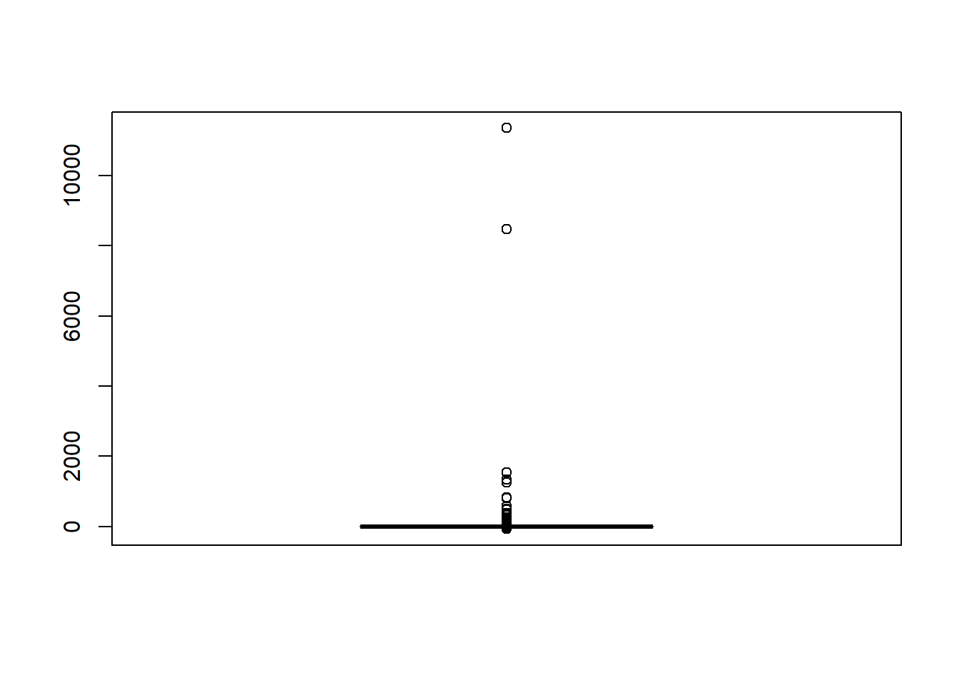

## model factors...
flist <- c('N1', 'N2', 'ICC_OV', 'ICC_LV', 'Estimator')
## Check assumptions
anova_assumptions_check(
  sdat, 'RB', factors = flist,
  model = as.formula('RB ~ N1 + N2 + ICC_OV + ICC_LV + Estimator + N1:N2 + N1:ICC_OV + N1:ICC_LV + N1:Estimator + N2:ICC_OV + N2:ICC_LV + N2:Estimator + ICC_OV:ICC_LV +  ICC_OV:Estimator  + ICC_LV:Estimator'))


 ============================= 

 Tests and Plots of Normality: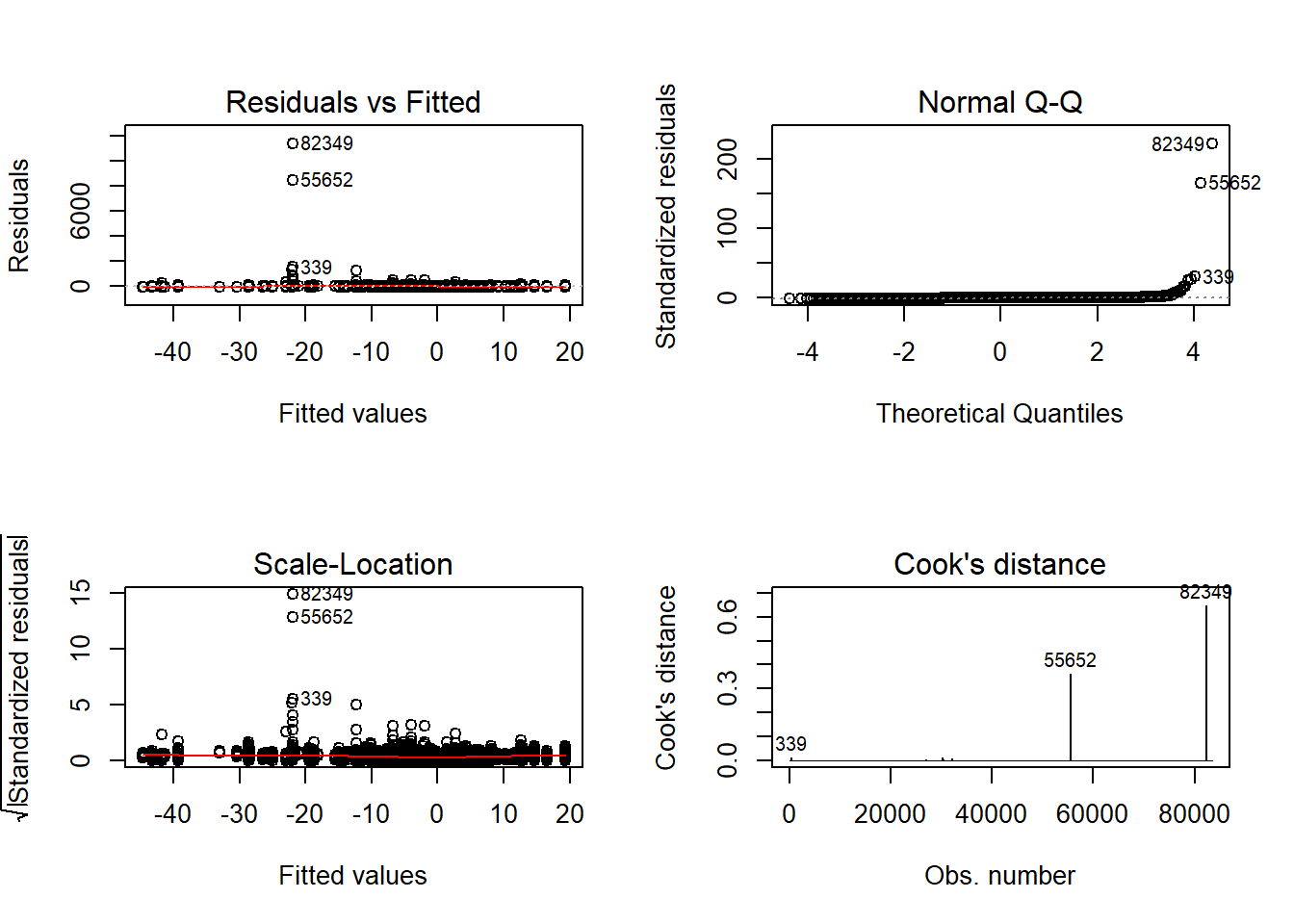


 Shapiro-Wilks Test of Normality of Residuals:

    Shapiro-Wilk normality test

data:  res
W = 0.9, p-value <2e-16


 K-S Test for Normality of Residuals:

    One-sample Kolmogorov-Smirnov test

data:  aov.out$residuals
D = 0.4, p-value <2e-16
alternative hypothesis: two-sided

`stat_bin()` using `bins = 30`. Pick better value with `binwidth`.

Warning: Removed 38 rows containing non-finite values (stat_bin).

Warning: Removed 3 rows containing missing values (geom_bar).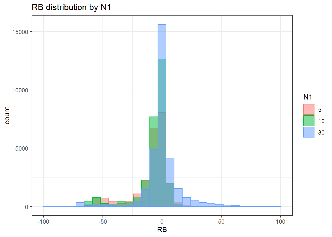

`stat_bin()` using `bins = 30`. Pick better value with `binwidth`.

Warning: Removed 38 rows containing non-finite values (stat_bin).

Warning: Removed 4 rows containing missing values (geom_bar).

`stat_bin()` using `bins = 30`. Pick better value with `binwidth`.

Warning: Removed 38 rows containing non-finite values (stat_bin).

Warning: Removed 3 rows containing missing values (geom_bar).

`stat_bin()` using `bins = 30`. Pick better value with `binwidth`.

Warning: Removed 38 rows containing non-finite values (stat_bin).

Warning: Removed 2 rows containing missing values (geom_bar).

`stat_bin()` using `bins = 30`. Pick better value with `binwidth`.

Warning: Removed 38 rows containing non-finite values (stat_bin).

Warning: Removed 3 rows containing missing values (geom_bar).


 ============================= 

 Tests of Homogeneity of Variance

 
 Levenes Test:  N1 
 
 
Levene's Test for Homogeneity of Variance (center = "mean")
         Df F value  Pr(>F)    
group     2    18.6 8.2e-09 ***
      83507                    
---
Signif. codes:  0 '***' 0.001 '**' 0.01 '*' 0.05 '.' 0.1 ' ' 1

 
 Levenes Test:  N2 
 
 
Levene's Test for Homogeneity of Variance (center = "mean")
         Df F value Pr(>F)    
group     3     100 <2e-16 ***
      83506                   
---
Signif. codes:  0 '***' 0.001 '**' 0.01 '*' 0.05 '.' 0.1 ' ' 1

 
 Levenes Test:  ICC_OV 
 
 
Levene's Test for Homogeneity of Variance (center = "mean")
         Df F value Pr(>F)    
group     2     556 <2e-16 ***
      83507                   
---
Signif. codes:  0 '***' 0.001 '**' 0.01 '*' 0.05 '.' 0.1 ' ' 1

 
 Levenes Test:  ICC_LV 
 
 
Levene's Test for Homogeneity of Variance (center = "mean")
         Df F value Pr(>F)    
group     1     451 <2e-16 ***
      83508                   
---
Signif. codes:  0 '***' 0.001 '**' 0.01 '*' 0.05 '.' 0.1 ' ' 1

 
 Levenes Test:  Estimator 
 
 
Levene's Test for Homogeneity of Variance (center = "mean")
         Df F value Pr(>F)    
group     2     628 <2e-16 ***
      83507                   
---
Signif. codes:  0 '***' 0.001 '**' 0.01 '*' 0.05 '.' 0.1 ' ' 1

# was bad... Remove extreme outliers
quantile(sdat$RB, c(0.001, 0.01, 0.99, 0.999))

 0.1%    1%   99% 99.9% 
-68.8 -60.1  36.2  76.9

# remove RB>100
sdat <- filter(sdat, RB <= 100)
boxplot(sdat$RB)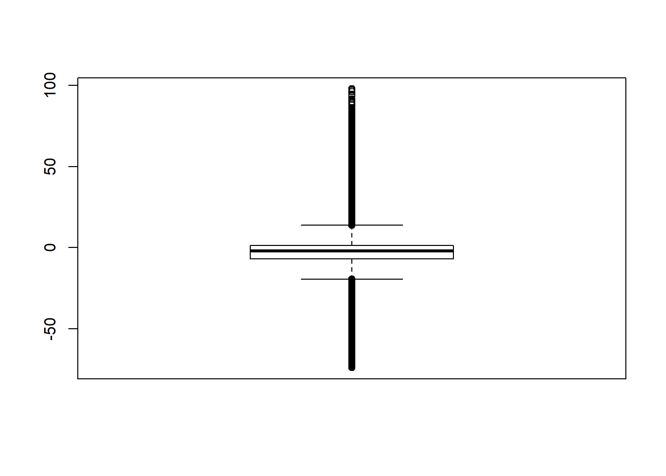

# rerun
## Check assumptions
anova_assumptions_check(
  sdat, 'RB', factors = flist,
  model = as.formula('RB ~ N1 + N2 + ICC_OV + ICC_LV + Estimator + N1:N2 + N1:ICC_OV + N1:ICC_LV + N1:Estimator + N2:ICC_OV + N2:ICC_LV + N2:Estimator + ICC_OV:ICC_LV +  ICC_OV:Estimator  + ICC_LV:Estimator'))


 ============================= 

 Tests and Plots of Normality: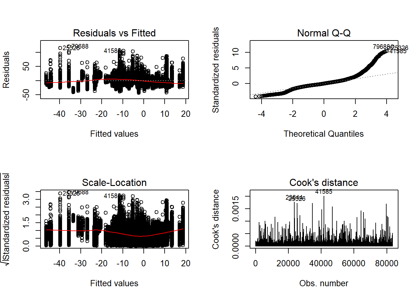


 Shapiro-Wilks Test of Normality of Residuals:

    Shapiro-Wilk normality test

data:  res
W = 0.9, p-value <2e-16


 K-S Test for Normality of Residuals:

    One-sample Kolmogorov-Smirnov test

data:  aov.out$residuals
D = 0.4, p-value <2e-16
alternative hypothesis: two-sided

`stat_bin()` using `bins = 30`. Pick better value with `binwidth`.

Warning: Removed 3 rows containing missing values (geom_bar).

`stat_bin()` using `bins = 30`. Pick better value with `binwidth`.

Warning: Removed 4 rows containing missing values (geom_bar).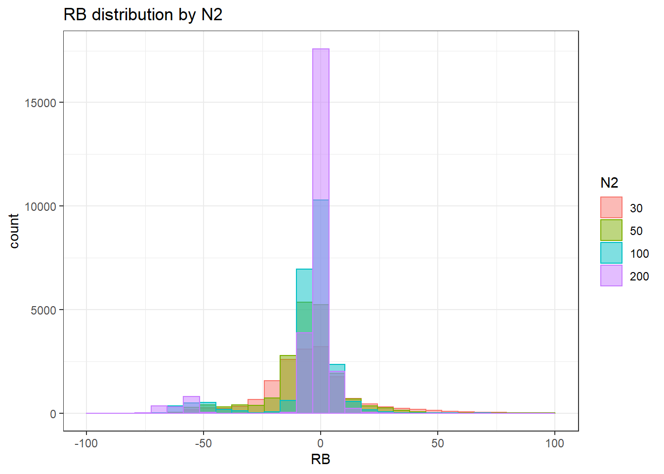

`stat_bin()` using `bins = 30`. Pick better value with `binwidth`.

Warning: Removed 3 rows containing missing values (geom_bar).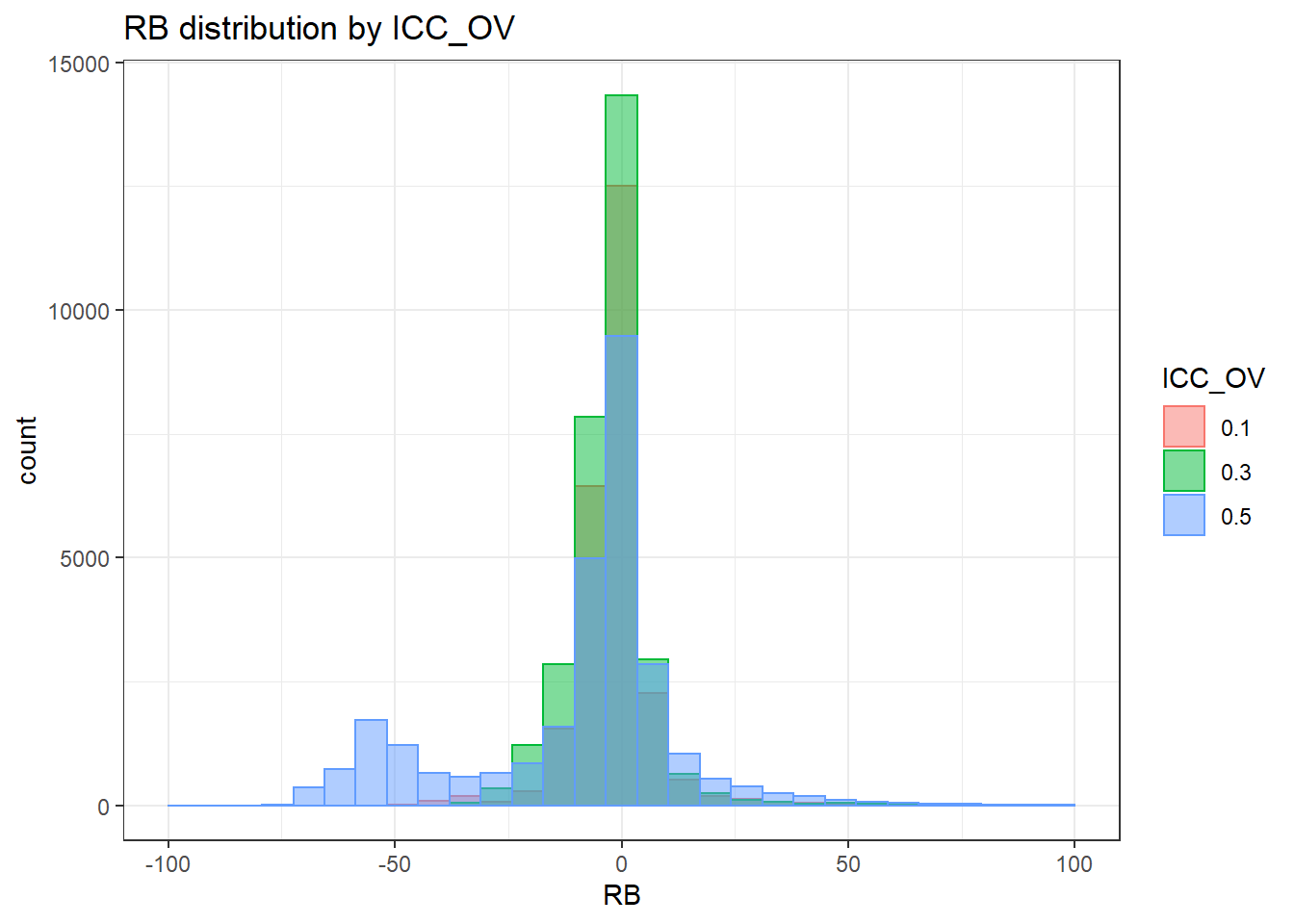

`stat_bin()` using `bins = 30`. Pick better value with `binwidth`.

Warning: Removed 2 rows containing missing values (geom_bar).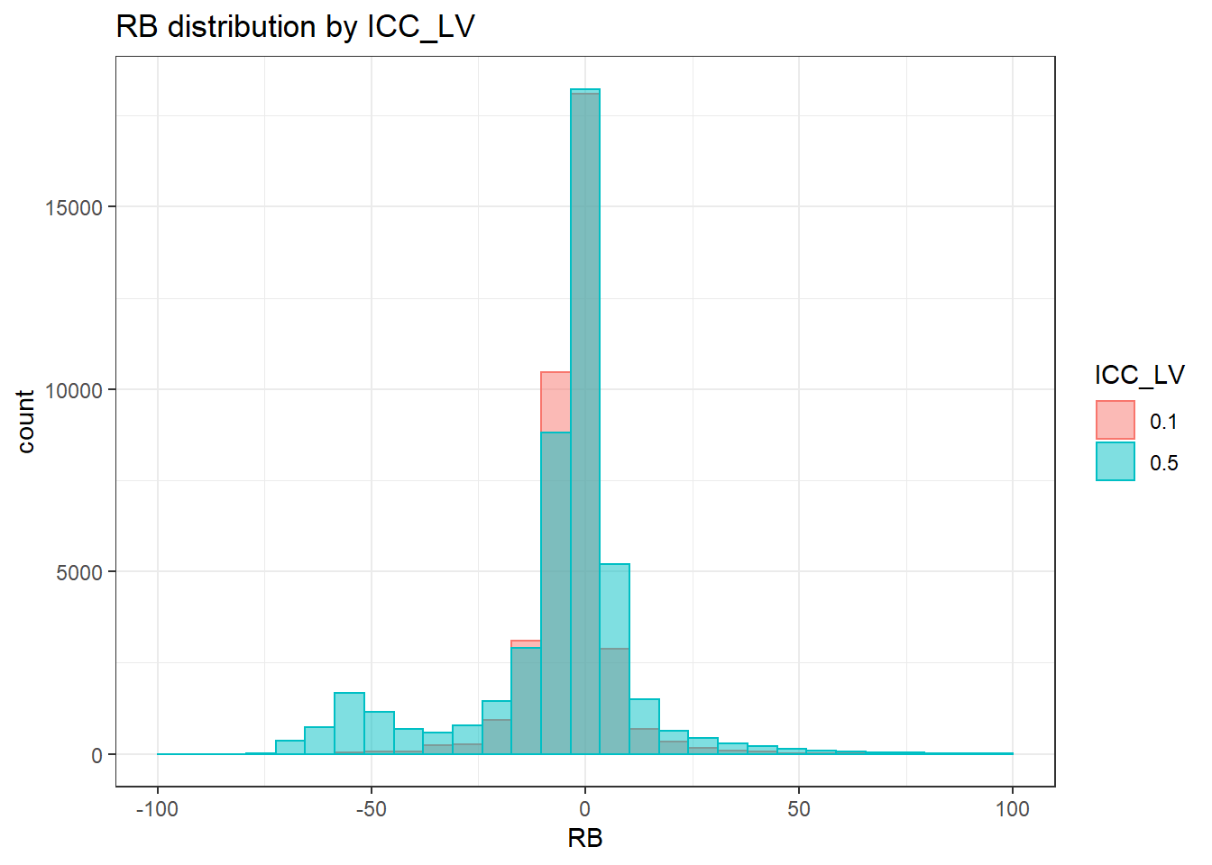

`stat_bin()` using `bins = 30`. Pick better value with `binwidth`.

Warning: Removed 3 rows containing missing values (geom_bar).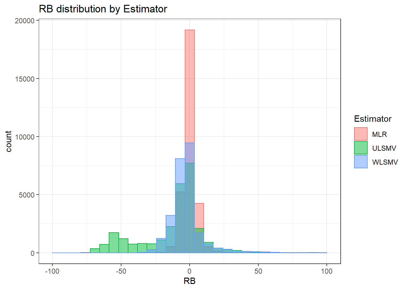


 ============================= 

 Tests of Homogeneity of Variance

 
 Levenes Test:  N1 
 
 
Levene's Test for Homogeneity of Variance (center = "mean")
         Df F value Pr(>F)    
group     2     167 <2e-16 ***
      83469                   
---
Signif. codes:  0 '***' 0.001 '**' 0.01 '*' 0.05 '.' 0.1 ' ' 1

 
 Levenes Test:  N2 
 
 
Levene's Test for Homogeneity of Variance (center = "mean")
         Df F value Pr(>F)    
group     3    1026 <2e-16 ***
      83468                   
---
Signif. codes:  0 '***' 0.001 '**' 0.01 '*' 0.05 '.' 0.1 ' ' 1

 
 Levenes Test:  ICC_OV 
 
 
Levene's Test for Homogeneity of Variance (center = "mean")
         Df F value Pr(>F)    
group     2   11697 <2e-16 ***
      83469                   
---
Signif. codes:  0 '***' 0.001 '**' 0.01 '*' 0.05 '.' 0.1 ' ' 1

 
 Levenes Test:  ICC_LV 
 
 
Levene's Test for Homogeneity of Variance (center = "mean")
         Df F value Pr(>F)    
group     1    7945 <2e-16 ***
      83470                   
---
Signif. codes:  0 '***' 0.001 '**' 0.01 '*' 0.05 '.' 0.1 ' ' 1

 
 Levenes Test:  Estimator 
 
 
Levene's Test for Homogeneity of Variance (center = "mean")
         Df F value Pr(>F)    
group     2   14504 <2e-16 ***
      83469                   
---
Signif. codes:  0 '***' 0.001 '**' 0.01 '*' 0.05 '.' 0.1 ' ' 1

ANOVA Results

model = as.formula('RB ~ N1 + N2 + ICC_OV + ICC_LV + Estimator + N1:N2 + N1:ICC_OV + N1:ICC_LV + N1:Estimator + N2:ICC_OV + N2:ICC_LV + N2:Estimator + ICC_OV:ICC_LV +  ICC_OV:Estimator  + ICC_LV:Estimator')

fit <- aov(model, data = sdat)
fit.out <- summary(fit)
fit.out

                    Df  Sum Sq Mean Sq F value Pr(>F)    
N1                   2 1047170  523585    5080 <2e-16 ***
N2                   3   67874   22625     220 <2e-16 ***
ICC_OV               2  891239  445620    4324 <2e-16 ***
ICC_LV               1  135863  135863    1318 <2e-16 ***
Estimator            2 2225371 1112686   10796 <2e-16 ***
N1:N2                6  500144   83357     809 <2e-16 ***
N1:ICC_OV            4  345837   86459     839 <2e-16 ***
N1:ICC_LV            2  111659   55830     542 <2e-16 ***
N1:Estimator         4  810663  202666    1966 <2e-16 ***
N2:ICC_OV            6  227670   37945     368 <2e-16 ***
N2:ICC_LV            3  344871  114957    1115 <2e-16 ***
N2:Estimator         6   70705   11784     114 <2e-16 ***
ICC_OV:ICC_LV        2  911306  455653    4421 <2e-16 ***
ICC_OV:Estimator     4 3632054  908013    8810 <2e-16 ***
ICC_LV:Estimator     2  684670  342335    3322 <2e-16 ***
Residuals        83422 8597901     103                   
---
Signif. codes:  0 '***' 0.001 '**' 0.01 '*' 0.05 '.' 0.1 ' ' 1

resultsList[["FactorLoadings"]] <- cbind(omega2(fit.out), p_omega2(fit.out))
resultsList[["FactorLoadings"]]

                 omega^2 partial-omega^2
N1                0.0508          0.1085
N2                0.0033          0.0078
ICC_OV            0.0432          0.0939
ICC_LV            0.0066          0.0155
Estimator         0.1080          0.2055
N1:N2             0.0242          0.0549
N1:ICC_OV         0.0168          0.0386
N1:ICC_LV         0.0054          0.0128
N1:Estimator      0.0393          0.0861
N2:ICC_OV         0.0110          0.0257
N2:ICC_LV         0.0167          0.0385
N2:Estimator      0.0034          0.0081
ICC_OV:ICC_LV     0.0442          0.0958
ICC_OV:Estimator  0.1762          0.2968
ICC_LV:Estimator  0.0332          0.0737

Level-1 factor Covariance Standard Error

Assumption Checking

sdat <- filter(long_results, Parameter %like% "psiW")

sdat <- sdat %>%
  group_by(Replication, N1, N2, ICC_OV, ICC_LV, Estimator) %>%
  summarise(RB = mean(RB))

# first, look at summary of RB Estimates
boxplot(sdat$RB)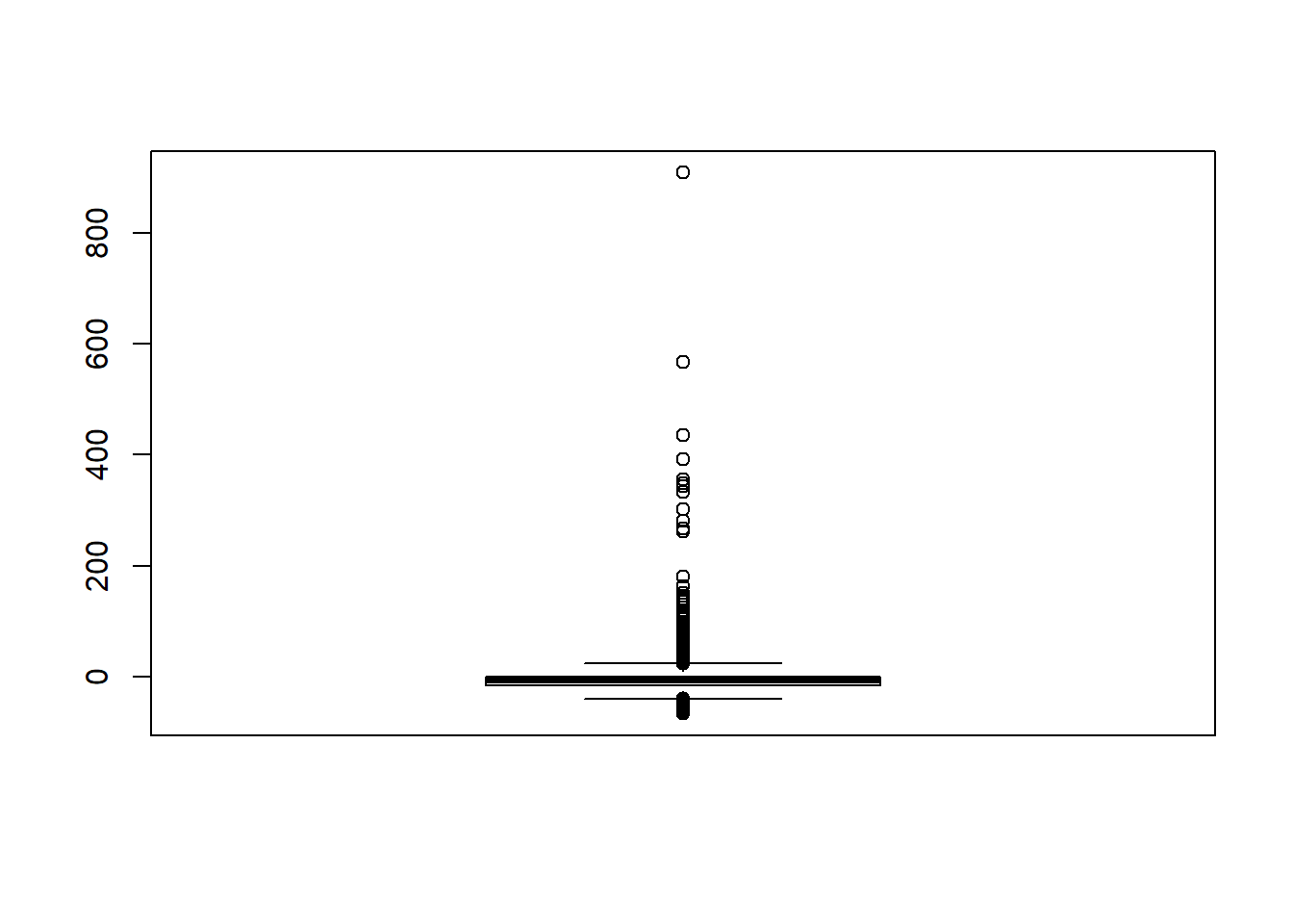

## model factors...
flist <- c('N1', 'N2', 'ICC_OV', 'ICC_LV', 'Estimator')
## Check assumptions
anova_assumptions_check(
  sdat, 'RB', factors = flist,
  model = as.formula('RB ~ N1 + N2 + ICC_OV + ICC_LV + Estimator + N1:N2 + N1:ICC_OV + N1:ICC_LV + N1:Estimator + N2:ICC_OV + N2:ICC_LV + N2:Estimator + ICC_OV:ICC_LV +  ICC_OV:Estimator  + ICC_LV:Estimator'))


 ============================= 

 Tests and Plots of Normality:


 Shapiro-Wilks Test of Normality of Residuals:

    Shapiro-Wilk normality test

data:  res
W = 0.8, p-value <2e-16


 K-S Test for Normality of Residuals:

Warning in ks.test(aov.out$residuals, "pnorm", alternative = "two.sided"): ties
should not be present for the Kolmogorov-Smirnov test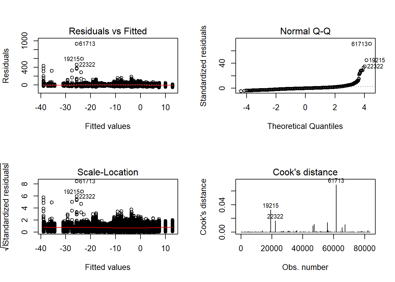


    One-sample Kolmogorov-Smirnov test

data:  aov.out$residuals
D = 0.4, p-value <2e-16
alternative hypothesis: two-sided

`stat_bin()` using `bins = 30`. Pick better value with `binwidth`.

Warning: Removed 30 rows containing non-finite values (stat_bin).

Warning: Removed 3 rows containing missing values (geom_bar).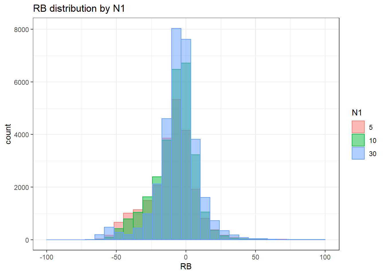

`stat_bin()` using `bins = 30`. Pick better value with `binwidth`.

Warning: Removed 30 rows containing non-finite values (stat_bin).

Warning: Removed 4 rows containing missing values (geom_bar).

`stat_bin()` using `bins = 30`. Pick better value with `binwidth`.

Warning: Removed 30 rows containing non-finite values (stat_bin).

Warning: Removed 3 rows containing missing values (geom_bar).

`stat_bin()` using `bins = 30`. Pick better value with `binwidth`.

Warning: Removed 30 rows containing non-finite values (stat_bin).

Warning: Removed 2 rows containing missing values (geom_bar).

`stat_bin()` using `bins = 30`. Pick better value with `binwidth`.

Warning: Removed 30 rows containing non-finite values (stat_bin).

Warning: Removed 3 rows containing missing values (geom_bar).


 ============================= 

 Tests of Homogeneity of Variance

 
 Levenes Test:  N1 
 
 
Levene's Test for Homogeneity of Variance (center = "mean")
         Df F value Pr(>F)    
group     2     249 <2e-16 ***
      83507                   
---
Signif. codes:  0 '***' 0.001 '**' 0.01 '*' 0.05 '.' 0.1 ' ' 1

 
 Levenes Test:  N2 
 
 
Levene's Test for Homogeneity of Variance (center = "mean")
         Df F value Pr(>F)    
group     3    2464 <2e-16 ***
      83506                   
---
Signif. codes:  0 '***' 0.001 '**' 0.01 '*' 0.05 '.' 0.1 ' ' 1

 
 Levenes Test:  ICC_OV 
 
 
Levene's Test for Homogeneity of Variance (center = "mean")
         Df F value Pr(>F)    
group     2    3328 <2e-16 ***
      83507                   
---
Signif. codes:  0 '***' 0.001 '**' 0.01 '*' 0.05 '.' 0.1 ' ' 1

 
 Levenes Test:  ICC_LV 
 
 
Levene's Test for Homogeneity of Variance (center = "mean")
         Df F value Pr(>F)    
group     1    2313 <2e-16 ***
      83508                   
---
Signif. codes:  0 '***' 0.001 '**' 0.01 '*' 0.05 '.' 0.1 ' ' 1

 
 Levenes Test:  Estimator 
 
 
Levene's Test for Homogeneity of Variance (center = "mean")
         Df F value Pr(>F)    
group     2    2414 <2e-16 ***
      83507                   
---
Signif. codes:  0 '***' 0.001 '**' 0.01 '*' 0.05 '.' 0.1 ' ' 1

# was bad... Remove extreme outliers
quantile(sdat$RB, c(0.001, 0.01, 0.99, 0.999))

 0.1%    1%   99% 99.9% 
-60.8 -52.7  29.4  67.2

# remove RB>100
sdat <- filter(sdat, RB <= 100)
boxplot(sdat$RB)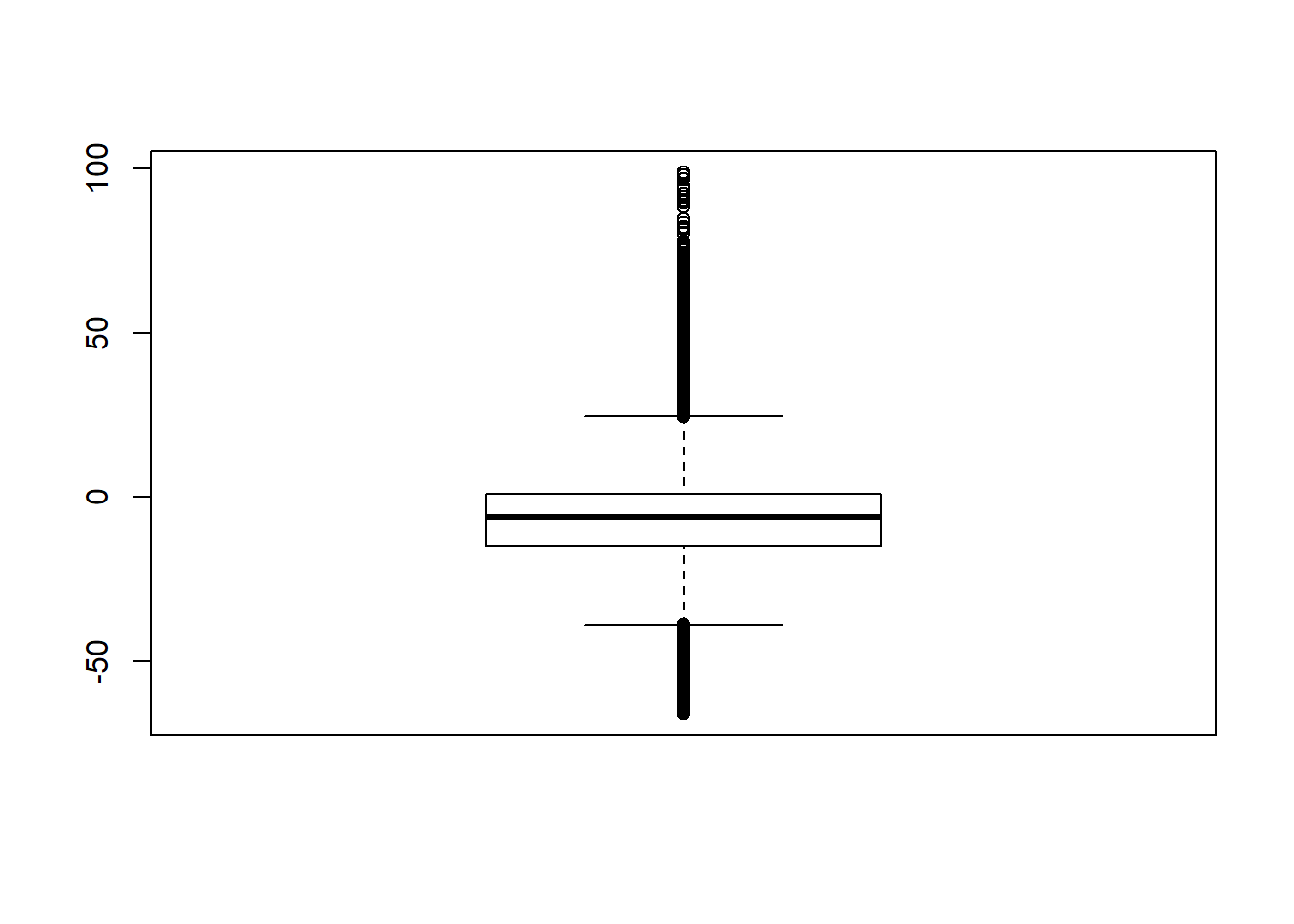

# rerun
## Check assumptions
anova_assumptions_check(
  sdat, 'RB', factors = flist,
  model = as.formula('RB ~ N1 + N2 + ICC_OV + ICC_LV + Estimator + N1:N2 + N1:ICC_OV + N1:ICC_LV + N1:Estimator + N2:ICC_OV + N2:ICC_LV + N2:Estimator + ICC_OV:ICC_LV +  ICC_OV:Estimator  + ICC_LV:Estimator'))


 ============================= 

 Tests and Plots of Normality:


 Shapiro-Wilks Test of Normality of Residuals:

    Shapiro-Wilk normality test

data:  res
W = 1, p-value <2e-16


 K-S Test for Normality of Residuals:

Warning in ks.test(aov.out$residuals, "pnorm", alternative = "two.sided"): ties
should not be present for the Kolmogorov-Smirnov test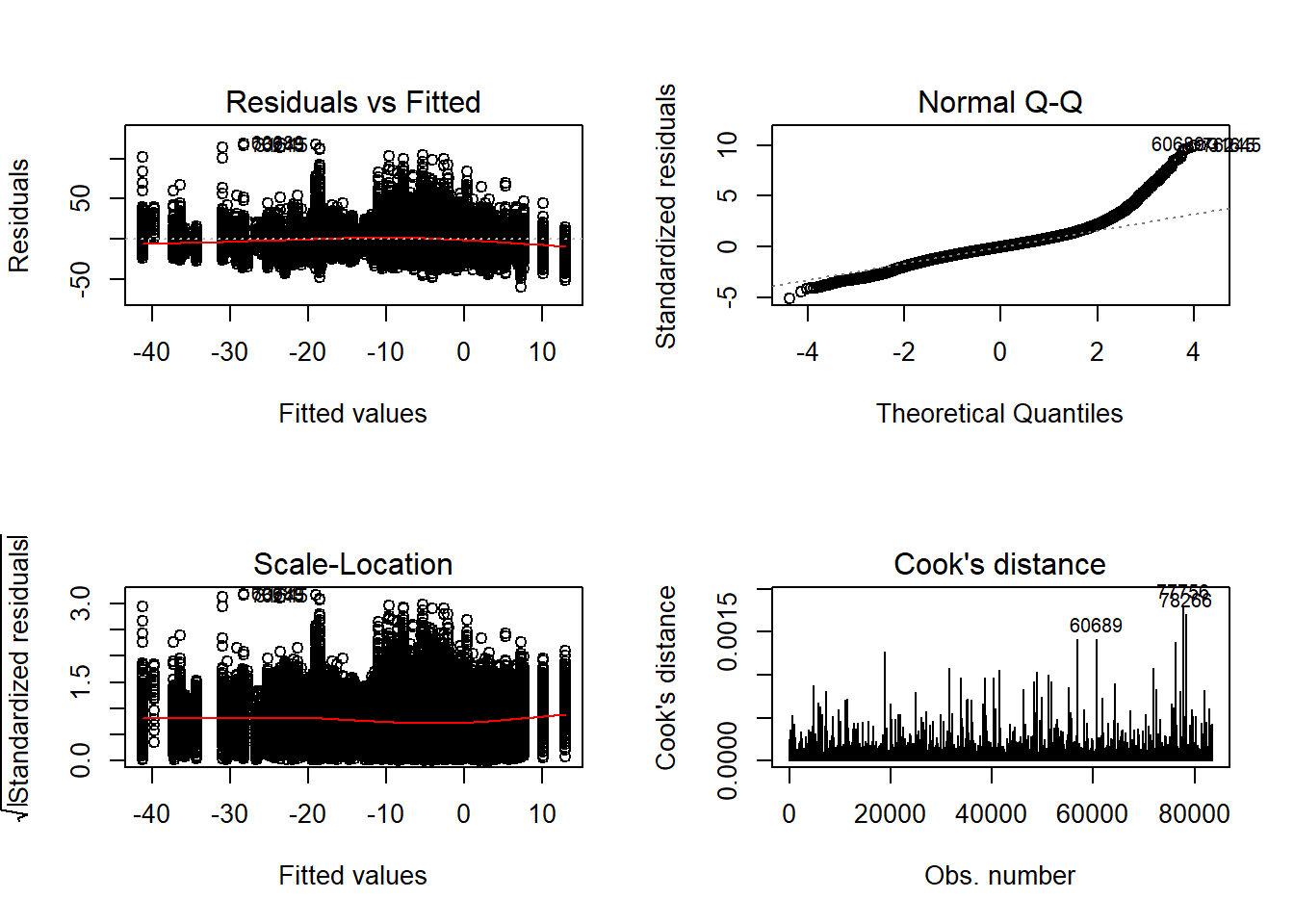


    One-sample Kolmogorov-Smirnov test

data:  aov.out$residuals
D = 0.4, p-value <2e-16
alternative hypothesis: two-sided

`stat_bin()` using `bins = 30`. Pick better value with `binwidth`.

Warning: Removed 3 rows containing missing values (geom_bar).

`stat_bin()` using `bins = 30`. Pick better value with `binwidth`.

Warning: Removed 4 rows containing missing values (geom_bar).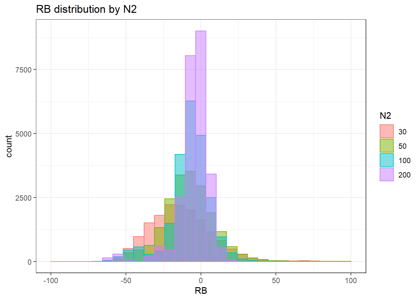

`stat_bin()` using `bins = 30`. Pick better value with `binwidth`.

Warning: Removed 3 rows containing missing values (geom_bar).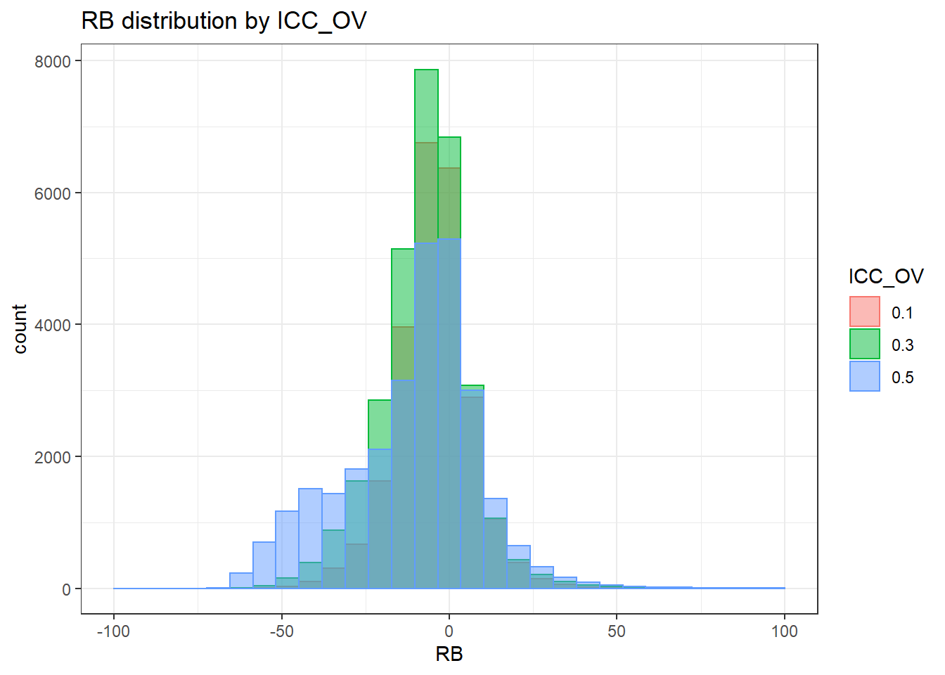

`stat_bin()` using `bins = 30`. Pick better value with `binwidth`.

Warning: Removed 2 rows containing missing values (geom_bar).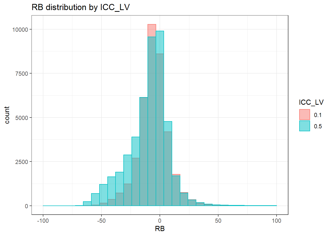

`stat_bin()` using `bins = 30`. Pick better value with `binwidth`.

Warning: Removed 3 rows containing missing values (geom_bar).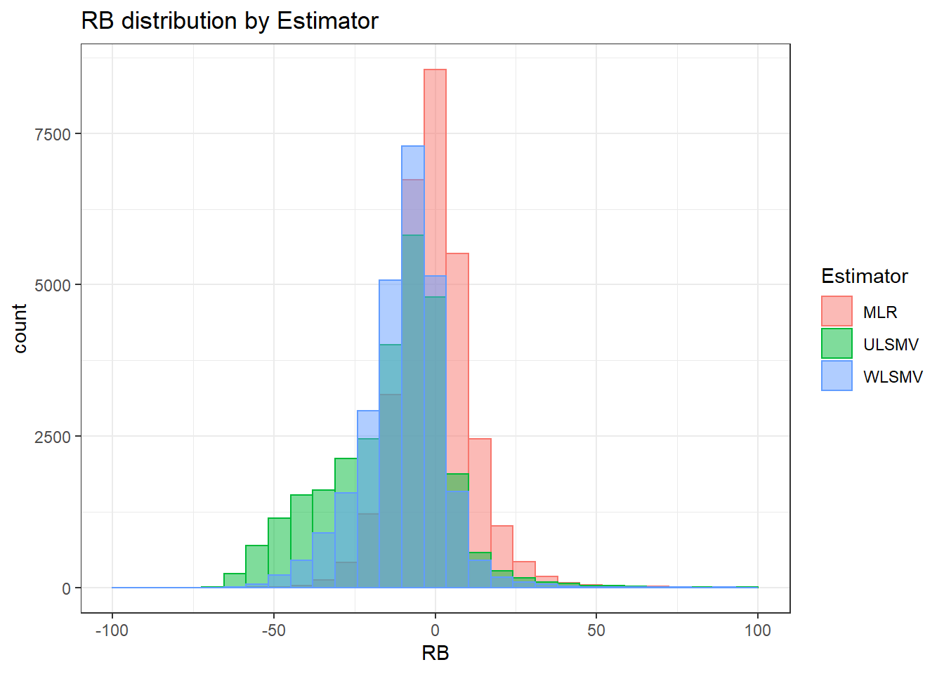


 ============================= 

 Tests of Homogeneity of Variance

 
 Levenes Test:  N1 
 
 
Levene's Test for Homogeneity of Variance (center = "mean")
         Df F value Pr(>F)    
group     2     264 <2e-16 ***
      83477                   
---
Signif. codes:  0 '***' 0.001 '**' 0.01 '*' 0.05 '.' 0.1 ' ' 1

 
 Levenes Test:  N2 
 
 
Levene's Test for Homogeneity of Variance (center = "mean")
         Df F value Pr(>F)    
group     3    2913 <2e-16 ***
      83476                   
---
Signif. codes:  0 '***' 0.001 '**' 0.01 '*' 0.05 '.' 0.1 ' ' 1

 
 Levenes Test:  ICC_OV 
 
 
Levene's Test for Homogeneity of Variance (center = "mean")
         Df F value Pr(>F)    
group     2    4179 <2e-16 ***
      83477                   
---
Signif. codes:  0 '***' 0.001 '**' 0.01 '*' 0.05 '.' 0.1 ' ' 1

 
 Levenes Test:  ICC_LV 
 
 
Levene's Test for Homogeneity of Variance (center = "mean")
         Df F value Pr(>F)    
group     1    2862 <2e-16 ***
      83478                   
---
Signif. codes:  0 '***' 0.001 '**' 0.01 '*' 0.05 '.' 0.1 ' ' 1

 
 Levenes Test:  Estimator 
 
 
Levene's Test for Homogeneity of Variance (center = "mean")
         Df F value Pr(>F)    
group     2    3242 <2e-16 ***
      83477                   
---
Signif. codes:  0 '***' 0.001 '**' 0.01 '*' 0.05 '.' 0.1 ' ' 1

ANOVA Results

model = as.formula('RB ~ N1 + N2 + ICC_OV + ICC_LV + Estimator + N1:N2 + N1:ICC_OV + N1:ICC_LV + N1:Estimator + N2:ICC_OV + N2:ICC_LV + N2:Estimator + ICC_OV:ICC_LV +  ICC_OV:Estimator  + ICC_LV:Estimator')

fit <- aov(model, data = sdat)
fit.out <- summary(fit)
fit.out

                    Df   Sum Sq Mean Sq F value Pr(>F)    
N1                   2   364315  182158    1326 <2e-16 ***
N2                   3   786435  262145    1908 <2e-16 ***
ICC_OV               2   382034  191017    1390 <2e-16 ***
ICC_LV               1   247444  247444    1801 <2e-16 ***
Estimator            2  2935157 1467578   10680 <2e-16 ***
N1:N2                6   609866  101644     740 <2e-16 ***
N1:ICC_OV            4   207109   51777     377 <2e-16 ***
N1:ICC_LV            2    29692   14846     108 <2e-16 ***
N1:Estimator         4   355914   88978     648 <2e-16 ***
N2:ICC_OV            6   174707   29118     212 <2e-16 ***
N2:ICC_LV            3   208686   69562     506 <2e-16 ***
N2:Estimator         6   542519   90420     658 <2e-16 ***
ICC_OV:ICC_LV        2   422966  211483    1539 <2e-16 ***
ICC_OV:Estimator     4  1132439  283110    2060 <2e-16 ***
ICC_LV:Estimator     2   333616  166808    1214 <2e-16 ***
Residuals        83430 11464454     137                   
---
Signif. codes:  0 '***' 0.001 '**' 0.01 '*' 0.05 '.' 0.1 ' ' 1

resultsList[["Level1-FactorCovariance"]] <- cbind(omega2(fit.out), p_omega2(fit.out))
resultsList[["Level1-FactorCovariance"]]

                 omega^2 partial-omega^2
N1                0.0180          0.0308
N2                0.0389          0.0641
ICC_OV            0.0189          0.0322
ICC_LV            0.0122          0.0211
Estimator         0.1453          0.2037
N1:N2             0.0302          0.0504
N1:ICC_OV         0.0102          0.0177
N1:ICC_LV         0.0015          0.0026
N1:Estimator      0.0176          0.0300
N2:ICC_OV         0.0086          0.0149
N2:ICC_LV         0.0103          0.0178
N2:Estimator      0.0268          0.0451
ICC_OV:ICC_LV     0.0209          0.0355
ICC_OV:Estimator  0.0560          0.0898
ICC_LV:Estimator  0.0165          0.0282

Level-2 factor (co)variances Standard Error

Assumption Checking

sdat <- filter(long_results, Parameter %like% "psiB")

sdat <- sdat %>%
  group_by(Replication, N1, N2, ICC_OV, ICC_LV, Estimator) %>%
  summarise(RB = mean(RB))

# first, look at summary of RB Estimates
boxplot(sdat$RB)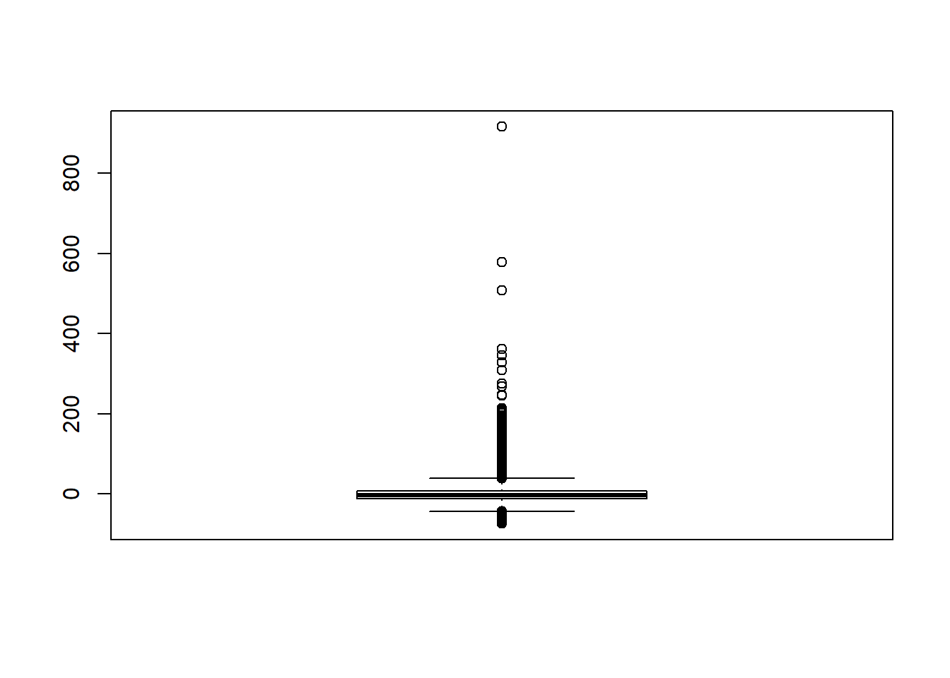

## model factors...
flist <- c('N1', 'N2', 'ICC_OV', 'ICC_LV', 'Estimator')
## Check assumptions
anova_assumptions_check(
  sdat, 'RB', factors = flist,
  model = as.formula('RB ~ N1 + N2 + ICC_OV + ICC_LV + Estimator + N1:N2 + N1:ICC_OV + N1:ICC_LV + N1:Estimator + N2:ICC_OV + N2:ICC_LV + N2:Estimator + ICC_OV:ICC_LV +  ICC_OV:Estimator  + ICC_LV:Estimator'))


 ============================= 

 Tests and Plots of Normality: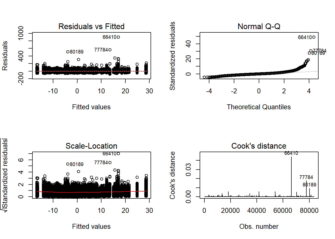


 Shapiro-Wilks Test of Normality of Residuals:

    Shapiro-Wilk normality test

data:  res
W = 0.9, p-value <2e-16


 K-S Test for Normality of Residuals:

    One-sample Kolmogorov-Smirnov test

data:  aov.out$residuals
D = 0.5, p-value <2e-16
alternative hypothesis: two-sided

`stat_bin()` using `bins = 30`. Pick better value with `binwidth`.

Warning: Removed 169 rows containing non-finite values (stat_bin).

Warning: Removed 3 rows containing missing values (geom_bar).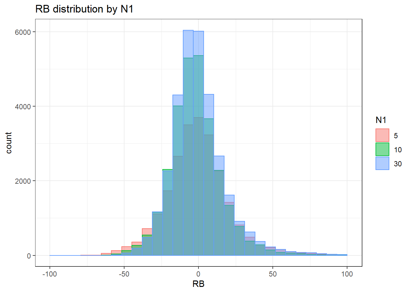

`stat_bin()` using `bins = 30`. Pick better value with `binwidth`.

Warning: Removed 169 rows containing non-finite values (stat_bin).

Warning: Removed 4 rows containing missing values (geom_bar).

`stat_bin()` using `bins = 30`. Pick better value with `binwidth`.

Warning: Removed 169 rows containing non-finite values (stat_bin).

Warning: Removed 3 rows containing missing values (geom_bar).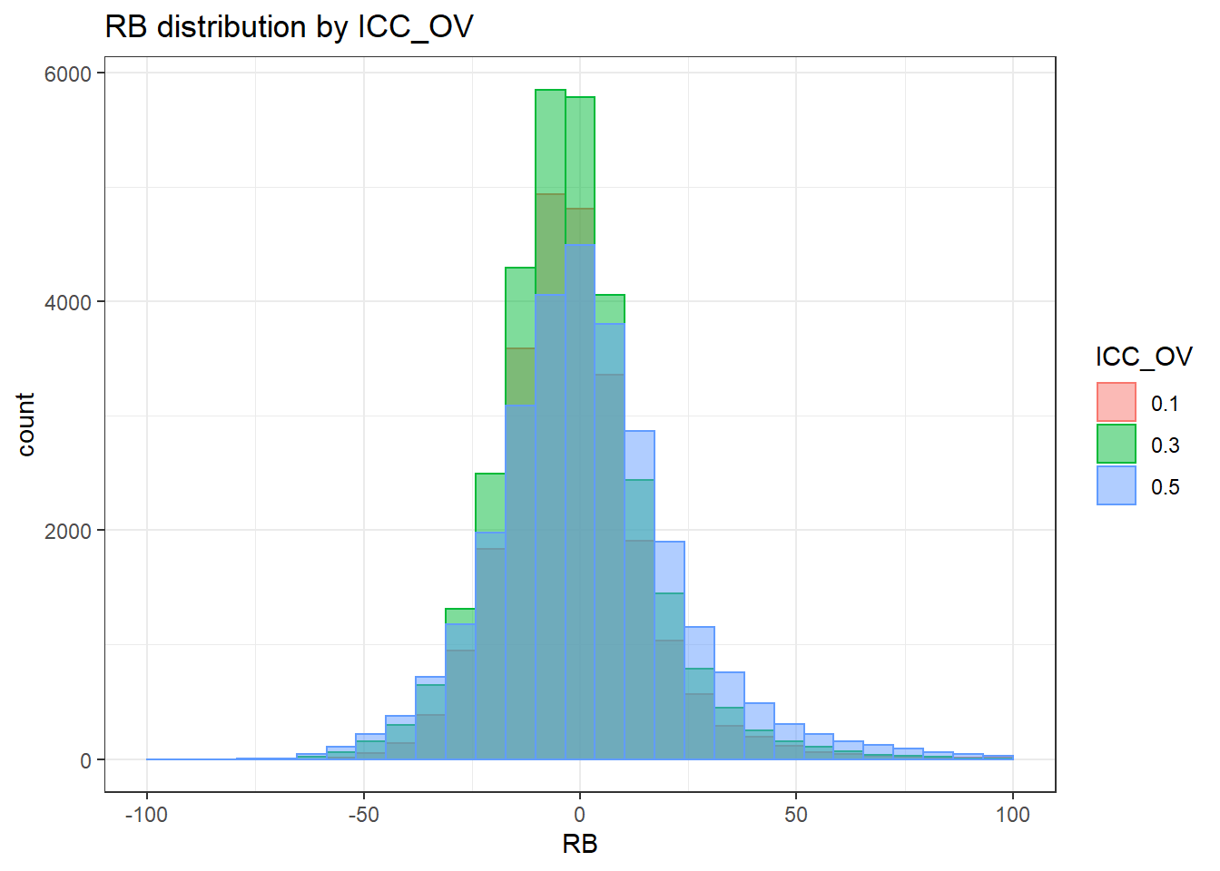

`stat_bin()` using `bins = 30`. Pick better value with `binwidth`.

Warning: Removed 169 rows containing non-finite values (stat_bin).

Warning: Removed 2 rows containing missing values (geom_bar).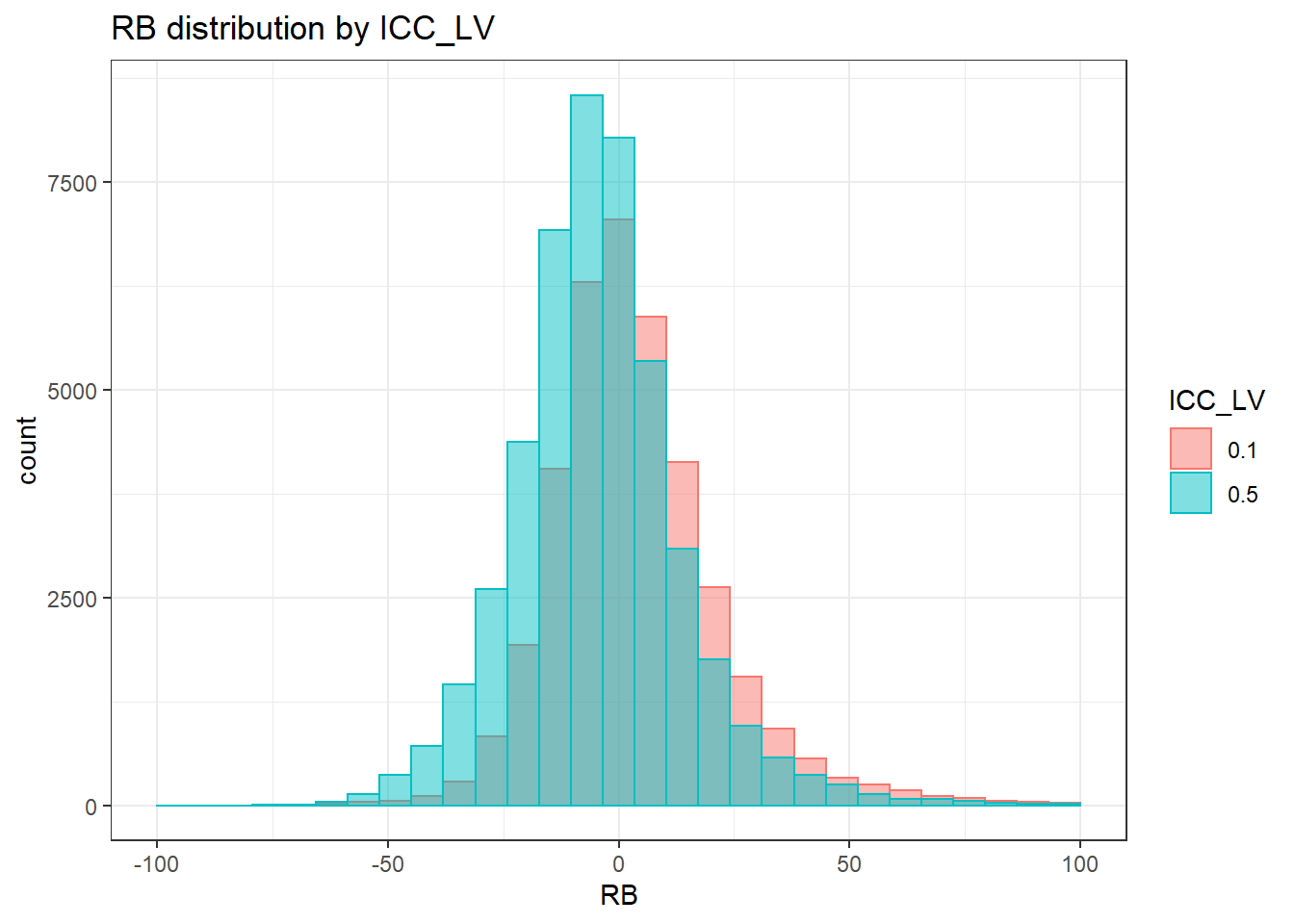

`stat_bin()` using `bins = 30`. Pick better value with `binwidth`.

Warning: Removed 169 rows containing non-finite values (stat_bin).

Warning: Removed 3 rows containing missing values (geom_bar).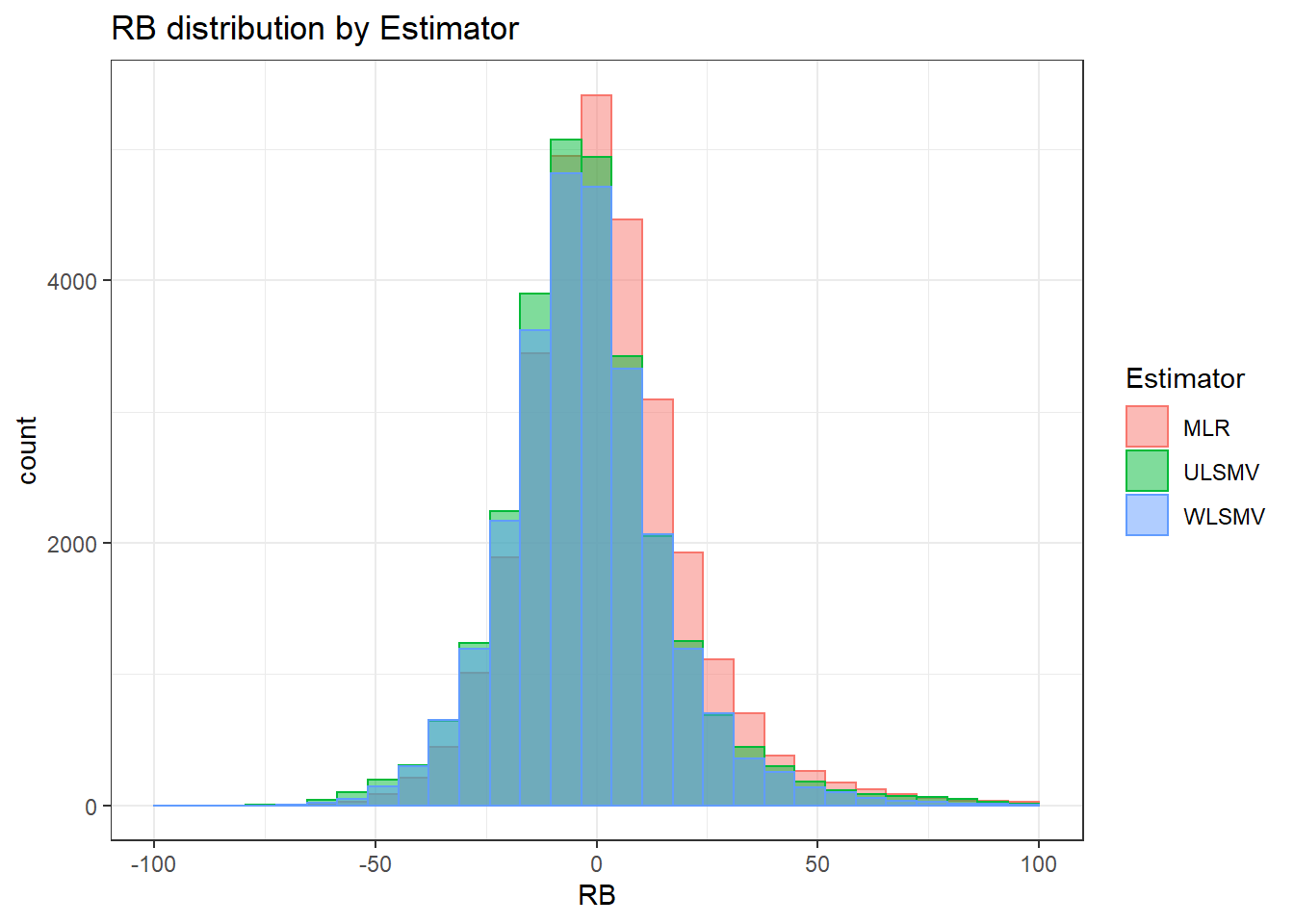


 ============================= 

 Tests of Homogeneity of Variance

 
 Levenes Test:  N1 
 
 
Levene's Test for Homogeneity of Variance (center = "mean")
         Df F value Pr(>F)    
group     2     423 <2e-16 ***
      83507                   
---
Signif. codes:  0 '***' 0.001 '**' 0.01 '*' 0.05 '.' 0.1 ' ' 1

 
 Levenes Test:  N2 
 
 
Levene's Test for Homogeneity of Variance (center = "mean")
         Df F value Pr(>F)    
group     3    4865 <2e-16 ***
      83506                   
---
Signif. codes:  0 '***' 0.001 '**' 0.01 '*' 0.05 '.' 0.1 ' ' 1

 
 Levenes Test:  ICC_OV 
 
 
Levene's Test for Homogeneity of Variance (center = "mean")
         Df F value Pr(>F)    
group     2     725 <2e-16 ***
      83507                   
---
Signif. codes:  0 '***' 0.001 '**' 0.01 '*' 0.05 '.' 0.1 ' ' 1

 
 Levenes Test:  ICC_LV 
 
 
Levene's Test for Homogeneity of Variance (center = "mean")
         Df F value  Pr(>F)    
group     1    30.5 3.3e-08 ***
      83508                    
---
Signif. codes:  0 '***' 0.001 '**' 0.01 '*' 0.05 '.' 0.1 ' ' 1

 
 Levenes Test:  Estimator 
 
 
Levene's Test for Homogeneity of Variance (center = "mean")
         Df F value Pr(>F)    
group     2    40.9 <2e-16 ***
      83507                   
---
Signif. codes:  0 '***' 0.001 '**' 0.01 '*' 0.05 '.' 0.1 ' ' 1

# was bad... Remove extreme outliers
quantile(sdat$RB, c(0.001, 0.01, 0.99, 0.999))

 0.1%    1%   99% 99.9% 
-57.8 -43.2  61.5 132.6

# remove RB>100
sdat <- filter(sdat, RB <= 100)
boxplot(sdat$RB)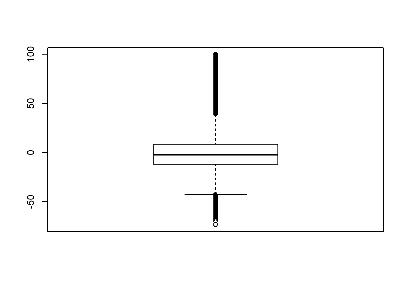

# rerun
## Check assumptions
anova_assumptions_check(
  sdat, 'RB', factors = flist,
  model = as.formula('RB ~ N1 + N2 + ICC_OV + ICC_LV + Estimator + N1:N2 + N1:ICC_OV + N1:ICC_LV + N1:Estimator + N2:ICC_OV + N2:ICC_LV + N2:Estimator + ICC_OV:ICC_LV +  ICC_OV:Estimator  + ICC_LV:Estimator'))


 ============================= 

 Tests and Plots of Normality: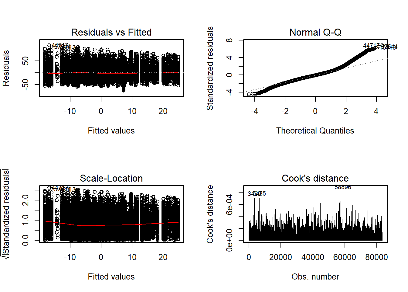


 Shapiro-Wilks Test of Normality of Residuals:

    Shapiro-Wilk normality test

data:  res
W = 1, p-value <2e-16


 K-S Test for Normality of Residuals:

    One-sample Kolmogorov-Smirnov test

data:  aov.out$residuals
D = 0.5, p-value <2e-16
alternative hypothesis: two-sided

`stat_bin()` using `bins = 30`. Pick better value with `binwidth`.

Warning: Removed 3 rows containing missing values (geom_bar).

`stat_bin()` using `bins = 30`. Pick better value with `binwidth`.

Warning: Removed 4 rows containing missing values (geom_bar).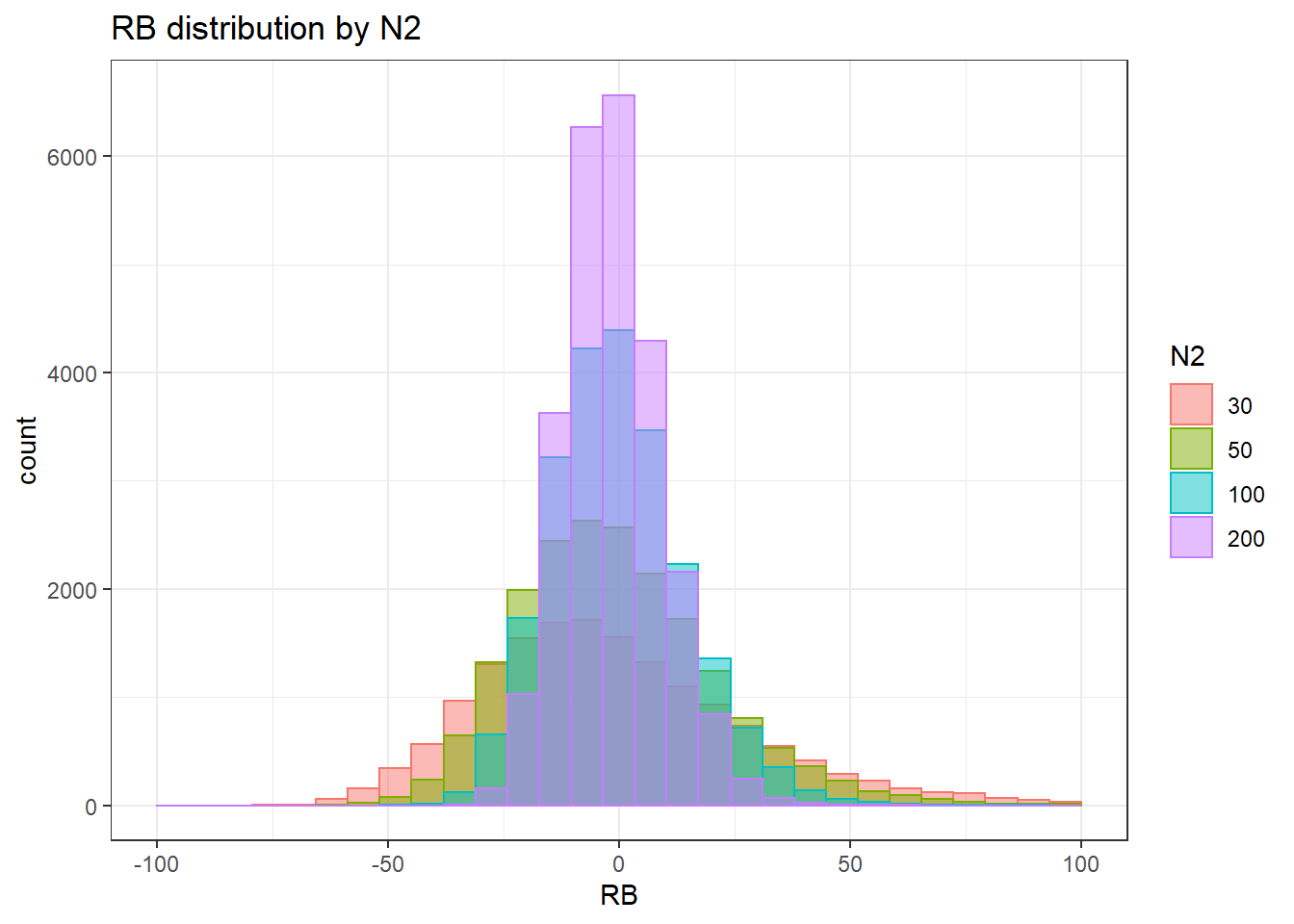

`stat_bin()` using `bins = 30`. Pick better value with `binwidth`.

Warning: Removed 3 rows containing missing values (geom_bar).

`stat_bin()` using `bins = 30`. Pick better value with `binwidth`.

Warning: Removed 2 rows containing missing values (geom_bar).

`stat_bin()` using `bins = 30`. Pick better value with `binwidth`.

Warning: Removed 3 rows containing missing values (geom_bar).


 ============================= 

 Tests of Homogeneity of Variance

 
 Levenes Test:  N1 
 
 
Levene's Test for Homogeneity of Variance (center = "mean")
         Df F value Pr(>F)    
group     2     402 <2e-16 ***
      83338                   
---
Signif. codes:  0 '***' 0.001 '**' 0.01 '*' 0.05 '.' 0.1 ' ' 1

 
 Levenes Test:  N2 
 
 
Levene's Test for Homogeneity of Variance (center = "mean")
         Df F value Pr(>F)    
group     3    5496 <2e-16 ***
      83337                   
---
Signif. codes:  0 '***' 0.001 '**' 0.01 '*' 0.05 '.' 0.1 ' ' 1

 
 Levenes Test:  ICC_OV 
 
 
Levene's Test for Homogeneity of Variance (center = "mean")
         Df F value Pr(>F)    
group     2     852 <2e-16 ***
      83338                   
---
Signif. codes:  0 '***' 0.001 '**' 0.01 '*' 0.05 '.' 0.1 ' ' 1

 
 Levenes Test:  ICC_LV 
 
 
Levene's Test for Homogeneity of Variance (center = "mean")
         Df F value Pr(>F)  
group     1    3.84   0.05 .
      83339                 
---
Signif. codes:  0 '***' 0.001 '**' 0.01 '*' 0.05 '.' 0.1 ' ' 1

 
 Levenes Test:  Estimator 
 
 
Levene's Test for Homogeneity of Variance (center = "mean")
         Df F value Pr(>F)    
group     2      23  1e-10 ***
      83338                   
---
Signif. codes:  0 '***' 0.001 '**' 0.01 '*' 0.05 '.' 0.1 ' ' 1

ANOVA Results

model = as.formula('RB ~ N1 + N2 + ICC_OV + ICC_LV + Estimator + N1:N2 + N1:ICC_OV + N1:ICC_LV + N1:Estimator + N2:ICC_OV + N2:ICC_LV + N2:Estimator + ICC_OV:ICC_LV +  ICC_OV:Estimator  + ICC_LV:Estimator')

fit <- aov(model, data = sdat)
fit.out <- summary(fit)
fit.out

                    Df   Sum Sq Mean Sq F value  Pr(>F)    
N1                   2    62807   31403   110.1 < 2e-16 ***
N2                   3    18825    6275    22.0 3.1e-14 ***
ICC_OV               2   257199  128600   450.7 < 2e-16 ***
ICC_LV               1  1504117 1504117  5271.9 < 2e-16 ***
Estimator            2   377801  188901   662.1 < 2e-16 ***
N1:N2                6   301046   50174   175.9 < 2e-16 ***
N1:ICC_OV            4   577371  144343   505.9 < 2e-16 ***
N1:ICC_LV            2   339801  169900   595.5 < 2e-16 ***
N1:Estimator         4   436345  109086   382.3 < 2e-16 ***
N2:ICC_OV            6    42861    7143    25.0 < 2e-16 ***
N2:ICC_LV            3   302766  100922   353.7 < 2e-16 ***
N2:Estimator         6    37316    6219    21.8 < 2e-16 ***
ICC_OV:ICC_LV        2   667850  333925  1170.4 < 2e-16 ***
ICC_OV:Estimator     4    11184    2796     9.8 6.4e-08 ***
ICC_LV:Estimator     2   132612   66306   232.4 < 2e-16 ***
Residuals        83291 23763672     285                    
---
Signif. codes:  0 '***' 0.001 '**' 0.01 '*' 0.05 '.' 0.1 ' ' 1

resultsList[["Level2-FactorCovariance"]] <- cbind(omega2(fit.out), p_omega2(fit.out))
resultsList[["Level2-FactorCovariance"]]

                 omega^2 partial-omega^2
N1                0.0022          0.0026
N2                0.0006          0.0008
ICC_OV            0.0089          0.0107
ICC_LV            0.0522          0.0595
Estimator         0.0131          0.0156
N1:N2             0.0104          0.0124
N1:ICC_OV         0.0200          0.0237
N1:ICC_LV         0.0118          0.0141
N1:Estimator      0.0151          0.0180
N2:ICC_OV         0.0014          0.0017
N2:ICC_LV         0.0105          0.0125
N2:Estimator      0.0012          0.0015
ICC_OV:ICC_LV     0.0231          0.0273
ICC_OV:Estimator  0.0003          0.0004
ICC_LV:Estimator  0.0046          0.0055

Level-2 item residual variances Standard Error

Assumption Checking

sdat <- filter(long_results, Parameter %like% "thetaB")

sdat <- sdat %>%
  group_by(Replication, N1, N2, ICC_OV, ICC_LV, Estimator) %>%
  summarise(RB = mean(RB))

# first, look at summary of RB Estimates
boxplot(sdat$RB)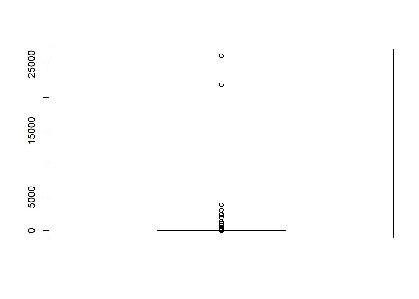

## model factors...
flist <- c('N1', 'N2', 'ICC_OV', 'ICC_LV', 'Estimator')
## Check assumptions
anova_assumptions_check(
  sdat, 'RB', factors = flist,
  model = as.formula('RB ~ N1 + N2 + ICC_OV + ICC_LV + Estimator + N1:N2 + N1:ICC_OV + N1:ICC_LV + N1:Estimator + N2:ICC_OV + N2:ICC_LV + N2:Estimator + ICC_OV:ICC_LV +  ICC_OV:Estimator  + ICC_LV:Estimator'))


 ============================= 

 Tests and Plots of Normality: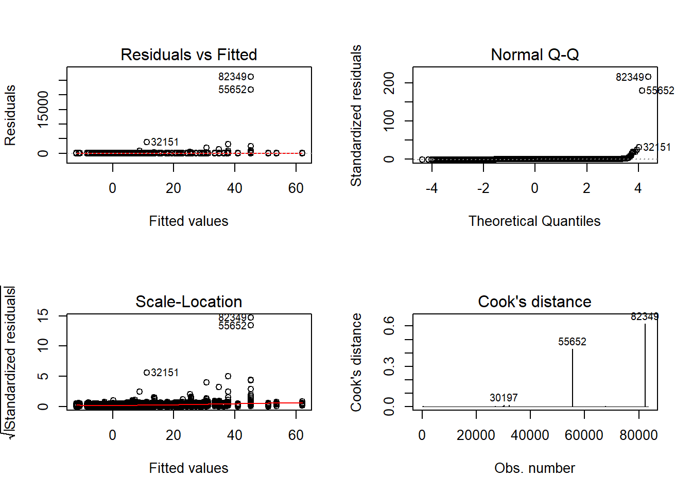


 Shapiro-Wilks Test of Normality of Residuals:

    Shapiro-Wilk normality test

data:  res
W = 0.09, p-value <2e-16


 K-S Test for Normality of Residuals:

    One-sample Kolmogorov-Smirnov test

data:  aov.out$residuals
D = 0.4, p-value <2e-16
alternative hypothesis: two-sided

`stat_bin()` using `bins = 30`. Pick better value with `binwidth`.

Warning: Removed 71 rows containing non-finite values (stat_bin).

Warning: Removed 3 rows containing missing values (geom_bar).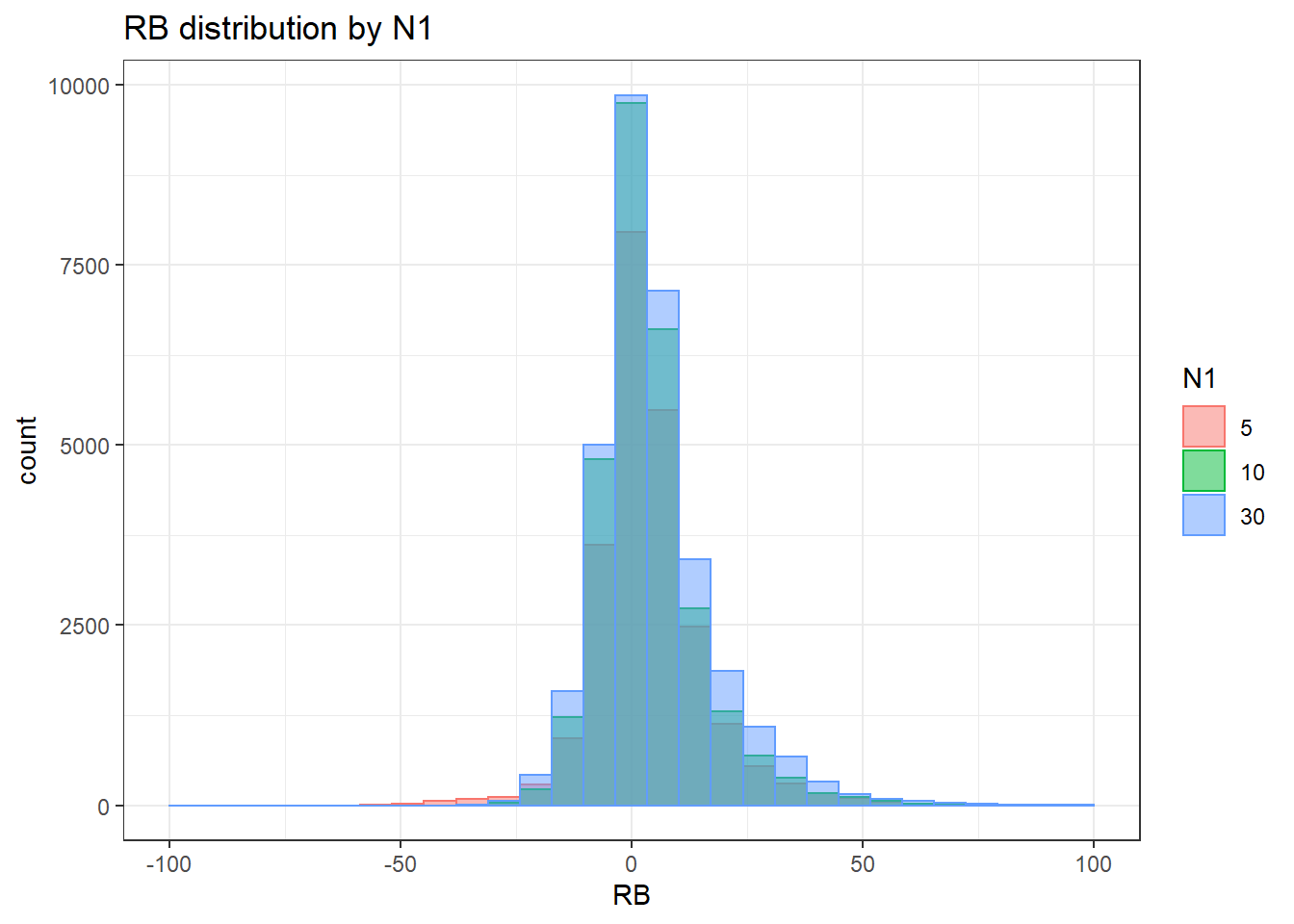

`stat_bin()` using `bins = 30`. Pick better value with `binwidth`.

Warning: Removed 71 rows containing non-finite values (stat_bin).

Warning: Removed 4 rows containing missing values (geom_bar).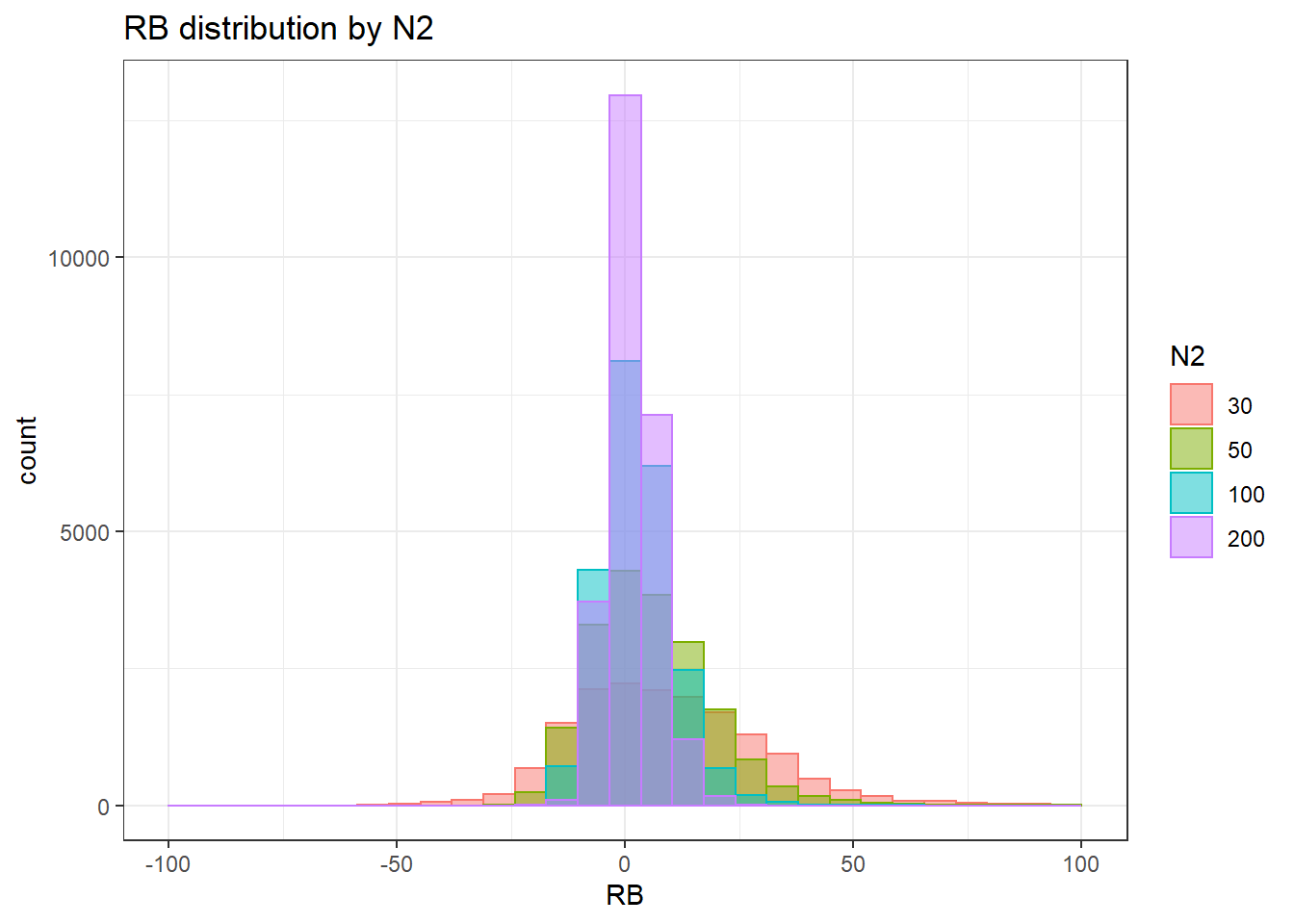

`stat_bin()` using `bins = 30`. Pick better value with `binwidth`.

Warning: Removed 71 rows containing non-finite values (stat_bin).

Warning: Removed 3 rows containing missing values (geom_bar).

`stat_bin()` using `bins = 30`. Pick better value with `binwidth`.

Warning: Removed 71 rows containing non-finite values (stat_bin).

Warning: Removed 2 rows containing missing values (geom_bar).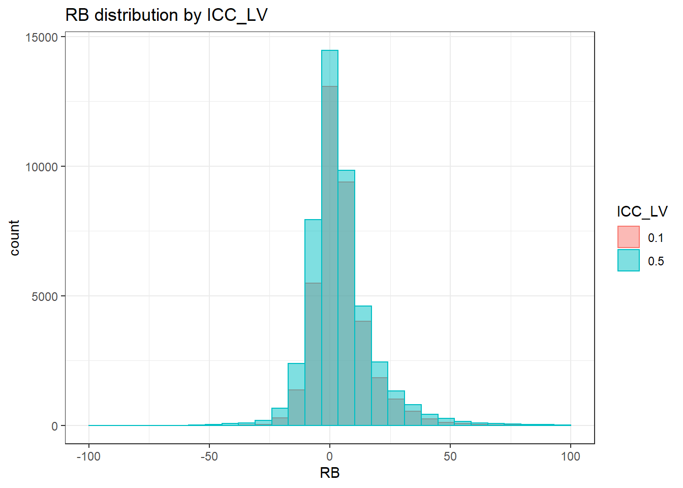

`stat_bin()` using `bins = 30`. Pick better value with `binwidth`.

Warning: Removed 71 rows containing non-finite values (stat_bin).

Warning: Removed 3 rows containing missing values (geom_bar).


 ============================= 

 Tests of Homogeneity of Variance

 
 Levenes Test:  N1 
 
 
Levene's Test for Homogeneity of Variance (center = "mean")
         Df F value Pr(>F)   
group     2    6.78 0.0011 **
      83507                  
---
Signif. codes:  0 '***' 0.001 '**' 0.01 '*' 0.05 '.' 0.1 ' ' 1

 
 Levenes Test:  N2 
 
 
Levene's Test for Homogeneity of Variance (center = "mean")
         Df F value Pr(>F)    
group     3      71 <2e-16 ***
      83506                   
---
Signif. codes:  0 '***' 0.001 '**' 0.01 '*' 0.05 '.' 0.1 ' ' 1

 
 Levenes Test:  ICC_OV 
 
 
Levene's Test for Homogeneity of Variance (center = "mean")
         Df F value Pr(>F)   
group     2    5.01 0.0067 **
      83507                  
---
Signif. codes:  0 '***' 0.001 '**' 0.01 '*' 0.05 '.' 0.1 ' ' 1

 
 Levenes Test:  ICC_LV 
 
 
Levene's Test for Homogeneity of Variance (center = "mean")
         Df F value  Pr(>F)    
group     1    15.3 9.3e-05 ***
      83508                    
---
Signif. codes:  0 '***' 0.001 '**' 0.01 '*' 0.05 '.' 0.1 ' ' 1

 
 Levenes Test:  Estimator 
 
 
Levene's Test for Homogeneity of Variance (center = "mean")
         Df F value  Pr(>F)    
group     2    23.8 4.9e-11 ***
      83507                    
---
Signif. codes:  0 '***' 0.001 '**' 0.01 '*' 0.05 '.' 0.1 ' ' 1

# was bad... Remove extreme outliers
quantile(sdat$RB, c(0.001, 0.01, 0.99, 0.999))

 0.1%    1%   99% 99.9% 
-38.6 -19.8  47.0  94.6

# remove RB>100
sdat <- filter(sdat, RB <= 100)
boxplot(sdat$RB)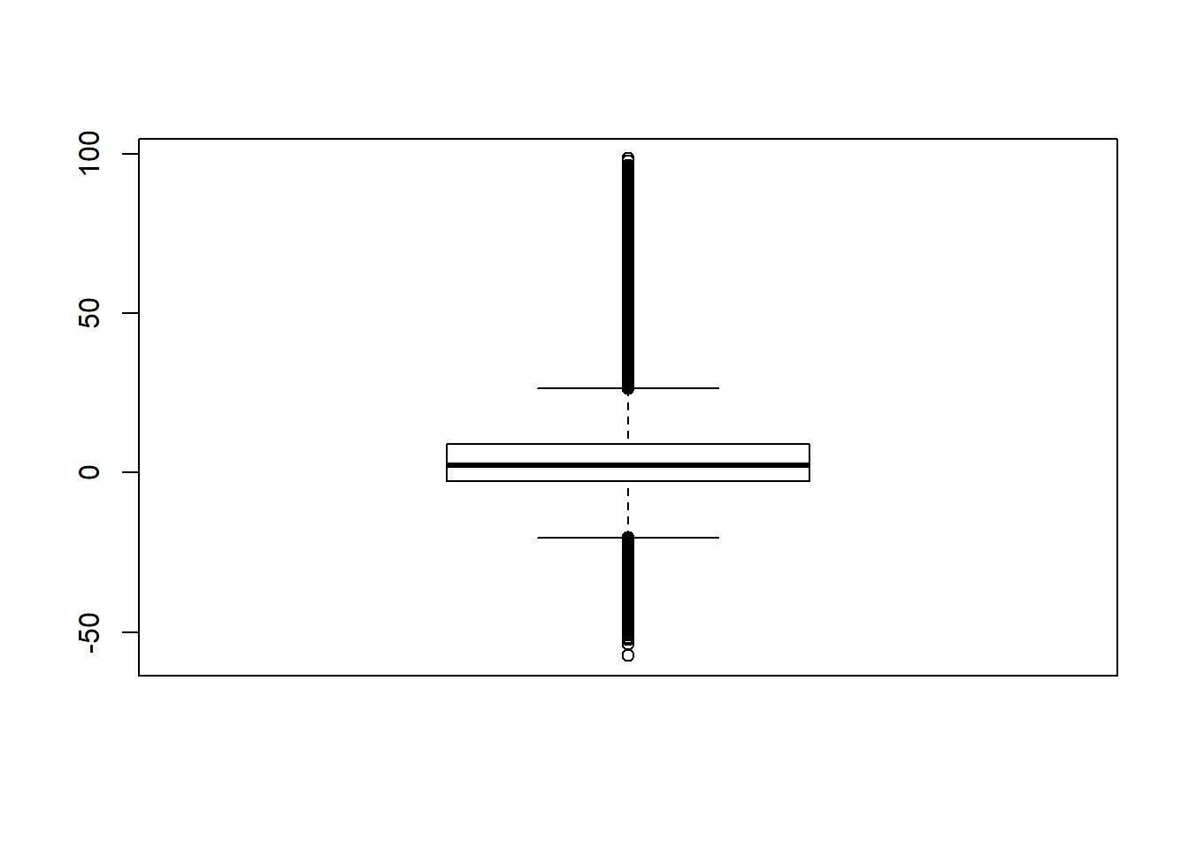

# rerun
## Check assumptions
anova_assumptions_check(
  sdat, 'RB', factors = flist,
  model = as.formula('RB ~ N1 + N2 + ICC_OV + ICC_LV + Estimator + N1:N2 + N1:ICC_OV + N1:ICC_LV + N1:Estimator + N2:ICC_OV + N2:ICC_LV + N2:Estimator + ICC_OV:ICC_LV +  ICC_OV:Estimator  + ICC_LV:Estimator'))


 ============================= 

 Tests and Plots of Normality: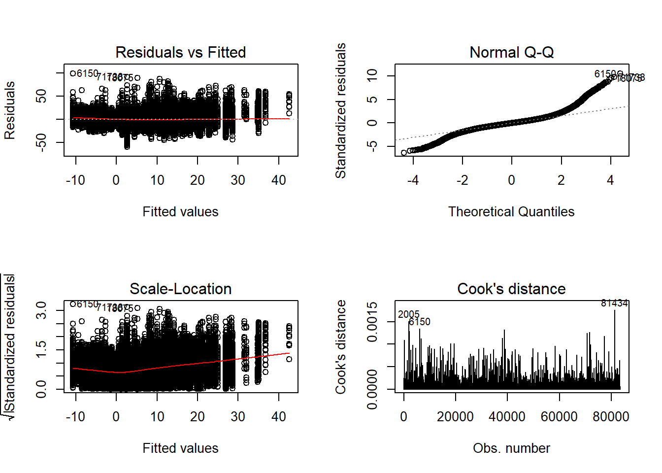


 Shapiro-Wilks Test of Normality of Residuals:

    Shapiro-Wilk normality test

data:  res
W = 0.9, p-value <2e-16


 K-S Test for Normality of Residuals:

    One-sample Kolmogorov-Smirnov test

data:  aov.out$residuals
D = 0.4, p-value <2e-16
alternative hypothesis: two-sided

`stat_bin()` using `bins = 30`. Pick better value with `binwidth`.

Warning: Removed 3 rows containing missing values (geom_bar).

`stat_bin()` using `bins = 30`. Pick better value with `binwidth`.

Warning: Removed 4 rows containing missing values (geom_bar).

`stat_bin()` using `bins = 30`. Pick better value with `binwidth`.

Warning: Removed 3 rows containing missing values (geom_bar).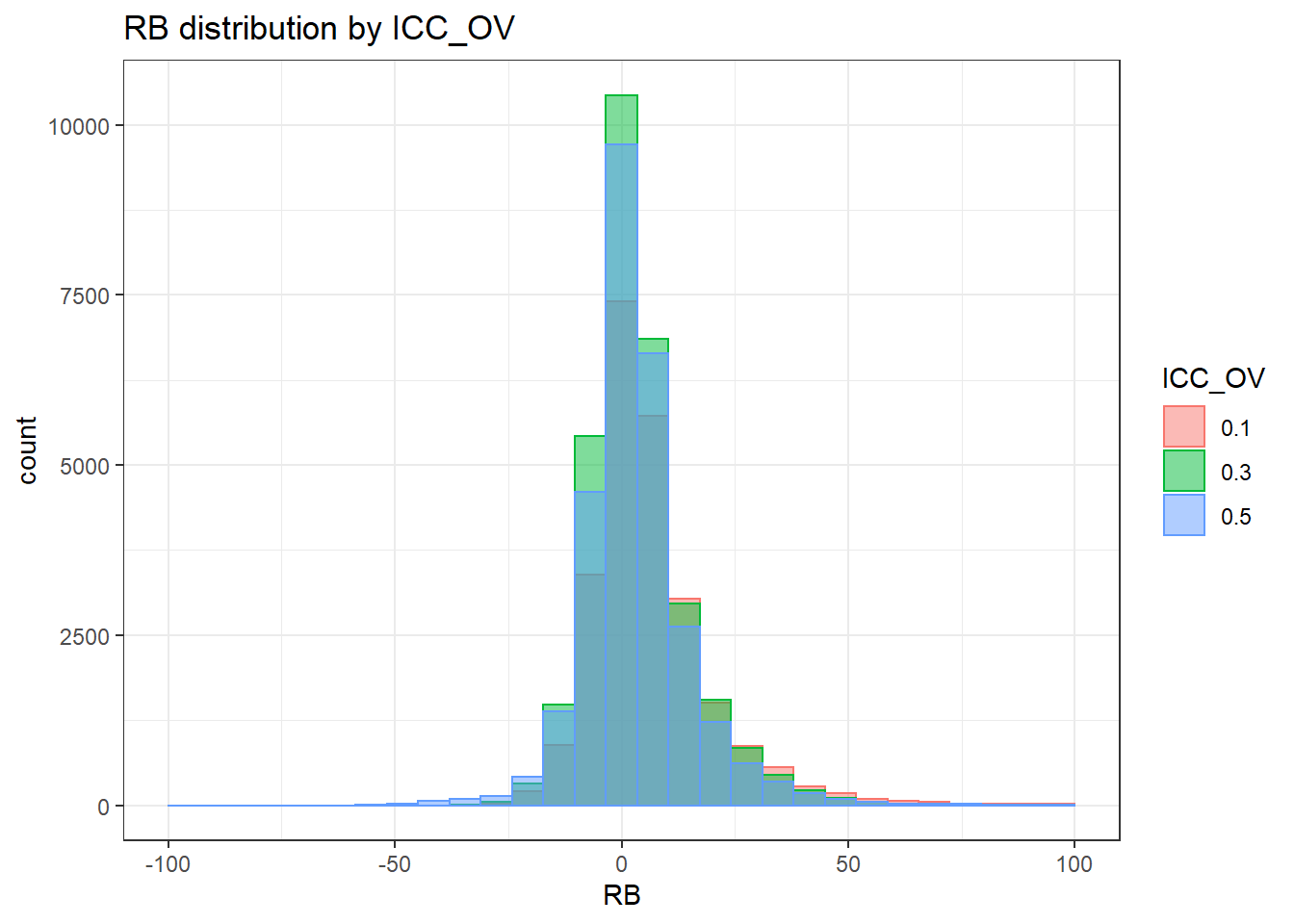

`stat_bin()` using `bins = 30`. Pick better value with `binwidth`.

Warning: Removed 2 rows containing missing values (geom_bar).

`stat_bin()` using `bins = 30`. Pick better value with `binwidth`.

Warning: Removed 3 rows containing missing values (geom_bar).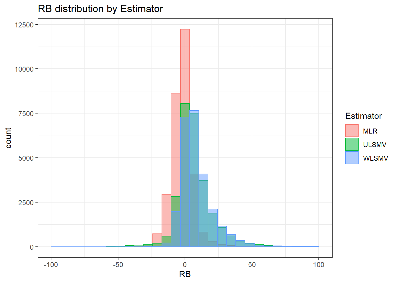


 ============================= 

 Tests of Homogeneity of Variance

 
 Levenes Test:  N1 
 
 
Levene's Test for Homogeneity of Variance (center = "mean")
         Df F value Pr(>F)    
group     2     157 <2e-16 ***
      83436                   
---
Signif. codes:  0 '***' 0.001 '**' 0.01 '*' 0.05 '.' 0.1 ' ' 1

 
 Levenes Test:  N2 
 
 
Levene's Test for Homogeneity of Variance (center = "mean")
         Df F value Pr(>F)    
group     3    9491 <2e-16 ***
      83435                   
---
Signif. codes:  0 '***' 0.001 '**' 0.01 '*' 0.05 '.' 0.1 ' ' 1

 
 Levenes Test:  ICC_OV 
 
 
Levene's Test for Homogeneity of Variance (center = "mean")
         Df F value Pr(>F)    
group     2     225 <2e-16 ***
      83436                   
---
Signif. codes:  0 '***' 0.001 '**' 0.01 '*' 0.05 '.' 0.1 ' ' 1

 
 Levenes Test:  ICC_LV 
 
 
Levene's Test for Homogeneity of Variance (center = "mean")
         Df F value Pr(>F)    
group     1     633 <2e-16 ***
      83437                   
---
Signif. codes:  0 '***' 0.001 '**' 0.01 '*' 0.05 '.' 0.1 ' ' 1

 
 Levenes Test:  Estimator 
 
 
Levene's Test for Homogeneity of Variance (center = "mean")
         Df F value Pr(>F)    
group     2    1735 <2e-16 ***
      83436                   
---
Signif. codes:  0 '***' 0.001 '**' 0.01 '*' 0.05 '.' 0.1 ' ' 1

ANOVA Results

model = as.formula('RB ~ N1 + N2 + ICC_OV + ICC_LV + Estimator + N1:N2 + N1:ICC_OV + N1:ICC_LV + N1:Estimator + N2:ICC_OV + N2:ICC_LV + N2:Estimator + ICC_OV:ICC_LV +  ICC_OV:Estimator  + ICC_LV:Estimator')

fit <- aov(model, data = sdat)
fit.out <- summary(fit)
fit.out

                    Df  Sum Sq Mean Sq F value  Pr(>F)    
N1                   2   25316   12658   141.9 < 2e-16 ***
N2                   3  609958  203319  2280.0 < 2e-16 ***
ICC_OV               2  214635  107318  1203.5 < 2e-16 ***
ICC_LV               1     508     508     5.7   0.017 *  
Estimator            2 2199362 1099681 12331.8 < 2e-16 ***
N1:N2                6   66553   11092   124.4 < 2e-16 ***
N1:ICC_OV            4  310637   77659   870.9 < 2e-16 ***
N1:ICC_LV            2     678     339     3.8   0.022 *  
N1:Estimator         4  159563   39891   447.3 < 2e-16 ***
N2:ICC_OV            6  227913   37985   426.0 < 2e-16 ***
N2:ICC_LV            3    2749     916    10.3 9.2e-07 ***
N2:Estimator         6  962350  160392  1798.6 < 2e-16 ***
ICC_OV:ICC_LV        2   94683   47342   530.9 < 2e-16 ***
ICC_OV:Estimator     4  112664   28166   315.9 < 2e-16 ***
ICC_LV:Estimator     2   64208   32104   360.0 < 2e-16 ***
Residuals        83389 7436157      89                    
---
Signif. codes:  0 '***' 0.001 '**' 0.01 '*' 0.05 '.' 0.1 ' ' 1

resultsList[["Level2-ResidualCovariance"]] <- cbind(omega2(fit.out), p_omega2(fit.out))
resultsList[["Level2-ResidualCovariance"]]

                 omega^2 partial-omega^2
N1                0.0020          0.0034
N2                0.0488          0.0757
ICC_OV            0.0172          0.0280
ICC_LV            0.0000          0.0001
Estimator         0.1761          0.2281
N1:N2             0.0053          0.0088
N1:ICC_OV         0.0248          0.0400
N1:ICC_LV         0.0000          0.0001
N1:Estimator      0.0127          0.0209
N2:ICC_OV         0.0182          0.0297
N2:ICC_LV         0.0002          0.0003
N2:Estimator      0.0770          0.1145
ICC_OV:ICC_LV     0.0076          0.0125
ICC_OV:Estimator  0.0090          0.0149
ICC_LV:Estimator  0.0051          0.0085

Summary Table of Effect Sizes

tb <- cbind(resultsList[[1]], resultsList[[2]], resultsList[[3]], resultsList[[4]])

kable(tb, format='html') %>%
    kable_styling(full_width = T) %>%
    add_header_above(c('Effect'=1,'Factor Loadings'=2,'Level-1 Factor Covariance'=2,'Level-2 Factor (co)variance'=2,'Level-2 Item Residual Variance'=2))

Effect	Factor Loadings		Level-1 Factor Covariance		Level-2 Factor (co)variance		Level-2 Item Residual Variance
	omega^2	partial-omega^2	omega^2	partial-omega^2	omega^2	partial-omega^2	omega^2	partial-omega^2
N1	0.051	0.108	0.018	0.031	0.002	0.003	0.002	0.003
N2	0.003	0.008	0.039	0.064	0.001	0.001	0.049	0.076
ICC_OV	0.043	0.094	0.019	0.032	0.009	0.011	0.017	0.028
ICC_LV	0.007	0.016	0.012	0.021	0.052	0.060	0.000	0.000
Estimator	0.108	0.206	0.145	0.204	0.013	0.016	0.176	0.228
N1:N2	0.024	0.055	0.030	0.050	0.010	0.012	0.005	0.009
N1:ICC_OV	0.017	0.039	0.010	0.018	0.020	0.024	0.025	0.040
N1:ICC_LV	0.005	0.013	0.002	0.003	0.012	0.014	0.000	0.000
N1:Estimator	0.039	0.086	0.018	0.030	0.015	0.018	0.013	0.021
N2:ICC_OV	0.011	0.026	0.009	0.015	0.001	0.002	0.018	0.030
N2:ICC_LV	0.017	0.038	0.010	0.018	0.010	0.012	0.000	0.000
N2:Estimator	0.003	0.008	0.027	0.045	0.001	0.002	0.077	0.114
ICC_OV:ICC_LV	0.044	0.096	0.021	0.036	0.023	0.027	0.008	0.012
ICC_OV:Estimator	0.176	0.297	0.056	0.090	0.000	0.000	0.009	0.015
ICC_LV:Estimator	0.033	0.074	0.016	0.028	0.005	0.006	0.005	0.008

## Print out in tex
print(xtable(tb, digits = 3), booktabs = T, include.rownames = T)

% latex table generated in R 3.6.3 by xtable 1.8-4 package
% Mon Jun 01 23:37:01 2020
\begin{table}[ht]
\centering
\begin{tabular}{rrrrrrrrr}
  \toprule
 & omega\verb|^|2 & partial-omega\verb|^|2 & omega\verb|^|2 & partial-omega\verb|^|2 & omega\verb|^|2 & partial-omega\verb|^|2 & omega\verb|^|2 & partial-omega\verb|^|2 \\ 
  \midrule
N1               & 0.051 & 0.108 & 0.018 & 0.031 & 0.002 & 0.003 & 0.002 & 0.003 \\ 
  N2               & 0.003 & 0.008 & 0.039 & 0.064 & 0.001 & 0.001 & 0.049 & 0.076 \\ 
  ICC\_OV           & 0.043 & 0.094 & 0.019 & 0.032 & 0.009 & 0.011 & 0.017 & 0.028 \\ 
  ICC\_LV           & 0.007 & 0.015 & 0.012 & 0.021 & 0.052 & 0.059 & 0.000 & 0.000 \\ 
  Estimator        & 0.108 & 0.205 & 0.145 & 0.204 & 0.013 & 0.016 & 0.176 & 0.228 \\ 
  N1:N2            & 0.024 & 0.055 & 0.030 & 0.050 & 0.010 & 0.012 & 0.005 & 0.009 \\ 
  N1:ICC\_OV        & 0.017 & 0.039 & 0.010 & 0.018 & 0.020 & 0.024 & 0.025 & 0.040 \\ 
  N1:ICC\_LV        & 0.005 & 0.013 & 0.002 & 0.003 & 0.012 & 0.014 & 0.000 & 0.000 \\ 
  N1:Estimator     & 0.039 & 0.086 & 0.018 & 0.030 & 0.015 & 0.018 & 0.013 & 0.021 \\ 
  N2:ICC\_OV        & 0.011 & 0.026 & 0.009 & 0.015 & 0.001 & 0.002 & 0.018 & 0.030 \\ 
  N2:ICC\_LV        & 0.017 & 0.038 & 0.010 & 0.018 & 0.010 & 0.012 & 0.000 & 0.000 \\ 
  N2:Estimator     & 0.003 & 0.008 & 0.027 & 0.045 & 0.001 & 0.002 & 0.077 & 0.114 \\ 
  ICC\_OV:ICC\_LV    & 0.044 & 0.096 & 0.021 & 0.035 & 0.023 & 0.027 & 0.008 & 0.012 \\ 
  ICC\_OV:Estimator & 0.176 & 0.297 & 0.056 & 0.090 & 0.000 & 0.000 & 0.009 & 0.015 \\ 
  ICC\_LV:Estimator & 0.033 & 0.074 & 0.016 & 0.028 & 0.005 & 0.005 & 0.005 & 0.008 \\ 
   \bottomrule
\end{tabular}
\end{table}

# ## Table of partial-omega2
# tb <- cbind(resultsList[[1]][,1, drop=F], resultsList[[2]][,1, drop=F], resultsList[[3]][,1, drop=F], resultsList[[4]][,1, drop=F])
# 
# kable(tb, format='html') %>%
#     kable_styling(full_width = T) %>%
#     add_header_above(c('Effect'=1,'Factor Loadings'=2,'Level-1 Factor Covariance'=2,'Level-2 Factor (co)variance'=2,'Level-2 Item Residual Variance'=2))
# 
# ## Print out in tex
# print(xtable(tb, digits = 3), booktabs = T, include.rownames = T)
# 
# 
# ## Table of omega-2
# tb <- cbind(resultsList[[1]][,1, drop=F], resultsList[[2]][,1, drop=F], resultsList[[3]][,1, drop=F], resultsList[[4]][,1, drop=F])
# 
# kable(tb, format='html') %>%
#     kable_styling(full_width = T) %>%
#     add_header_above(c('Effect'=1,'Factor Loadings'=2,'Level-1 Factor Covariance'=2,'Level-2 Factor (co)variance'=2,'Level-2 Item Residual Variance'=2))
# 
# ## Print out in tex
# print(xtable(tb, digits = 3), booktabs = T, include.rownames = T)

sessionInfo()

R version 3.6.3 (2020-02-29)
Platform: x86_64-w64-mingw32/x64 (64-bit)
Running under: Windows 10 x64 (build 18362)

Matrix products: default

locale:
[1] LC_COLLATE=English_United States.1252 
[2] LC_CTYPE=English_United States.1252   
[3] LC_MONETARY=English_United States.1252
[4] LC_NUMERIC=C                          
[5] LC_TIME=English_United States.1252    

attached base packages:
[1] stats     graphics  grDevices utils     datasets  methods   base     

other attached packages:
 [1] xtable_1.8-4          kableExtra_1.1.0      cowplot_1.0.0        
 [4] MplusAutomation_0.7-3 data.table_1.12.8     patchwork_1.0.0      
 [7] forcats_0.5.0         stringr_1.4.0         dplyr_0.8.5          
[10] purrr_0.3.4           readr_1.3.1           tidyr_1.1.0          
[13] tibble_3.0.1          ggplot2_3.3.0         tidyverse_1.3.0      
[16] workflowr_1.6.2      

loaded via a namespace (and not attached):
 [1] nlme_3.1-144      fs_1.4.1          lubridate_1.7.8   webshot_0.5.2    
 [5] httr_1.4.1        rprojroot_1.3-2   tools_3.6.3       backports_1.1.7  
 [9] R6_2.4.1          DBI_1.1.0         colorspace_1.4-1  withr_2.2.0      
[13] tidyselect_1.1.0  curl_4.3          compiler_3.6.3    git2r_0.27.1     
[17] cli_2.0.2         rvest_0.3.5       xml2_1.3.2        labeling_0.3     
[21] scales_1.1.1      digest_0.6.25     foreign_0.8-75    rmarkdown_2.1    
[25] rio_0.5.16        pkgconfig_2.0.3   htmltools_0.4.0   highr_0.8        
[29] dbplyr_1.4.4      rlang_0.4.6       readxl_1.3.1      rstudioapi_0.11  
[33] generics_0.0.2    farver_2.0.3      jsonlite_1.6.1    zip_2.0.4        
[37] car_3.0-8         magrittr_1.5      texreg_1.36.23    Rcpp_1.0.4.6     
[41] munsell_0.5.0     fansi_0.4.1       abind_1.4-5       proto_1.0.0      
[45] lifecycle_0.2.0   stringi_1.4.6     yaml_2.2.1        carData_3.0-4    
[49] plyr_1.8.6        grid_3.6.3        blob_1.2.1        parallel_3.6.3   
[53] promises_1.1.0    crayon_1.3.4      lattice_0.20-38   haven_2.3.0      
[57] pander_0.6.3      hms_0.5.3         knitr_1.28        pillar_1.4.4     
[61] boot_1.3-24       reprex_0.3.0      glue_1.4.1        evaluate_0.14    
[65] modelr_0.1.8      vctrs_0.3.0       httpuv_1.5.2      cellranger_1.1.0 
[69] gtable_0.3.0      assertthat_0.2.1  gsubfn_0.7        xfun_0.14        
[73] openxlsx_4.1.5    broom_0.5.6       coda_0.19-3       later_1.0.0      
[77] viridisLite_0.3.0 ellipsis_0.3.1

Design Effects on Standard Error Relative Bias Estimates

2020-06-01

Packages and Set-Up

Data Management

ANOVA and effect sizes for distributional differences

Factor Loadings Standard Error

Assumption Checking

ANOVA Results

Level-1 factor Covariance Standard Error

Assumption Checking

ANOVA Results

Level-2 factor (co)variances Standard Error

Assumption Checking

ANOVA Results

Level-2 item residual variances Standard Error

Assumption Checking

ANOVA Results

Summary Table of Effect Sizes