2 Introduction to Bayesian Inference
Chapter 2 is focused on introducing the fundamentals of Bayesian modeling. I will briefly reiterate some of these concepts, but Levy and Mislevy did an excellent job introducing the basic concepts so I defer to them. A few points I would like to highlight are
-
The concept of likelihood is fundamental to Bayesian methods and frequentist methods as well.
The likelihood function (denoted \(p(\mathbf{x} \mid \theta)\) or equivalently \(L(\theta \mid \mathbf{x})\)) is fundamental as this conditional probability describes our beliefs about the data generating process. Another way of thinking about the likelihood function is as the data model. The data model decribes how parameters of interest relates to the observed data. This key concept is used in frequentist methods (e.g., maximum likelihood estimation) to obtain point estimates of model parameters. A fundamental difference between maximum likelihood and Bayesian estimation is how we use the likelihood function to construct interval estimates of parameters (see next point).
-
Interval estimates in Bayesian methods do not rely on the idea of repeated sampling.
In frequentist analyses, the construction of interval estimates around maximum likelihood estimators is dependent on utilizing repeated sampling paradigm. The interval estimate around the MLE is referred to the sampling distribution of the parameter estimator. BPM discusses these features of maximum likelihood well on p. 26. In Bayesian methods, an interval estimate is constructed based on the distribution of the parameter and not the parameter estimator. This distinction makes Bayesian intervals based on the likely values of the parameter based on our prior beliefs and observed data.
-
Bayes Theorem
Bayes theorem is the underlying engine of all Bayesian methods. We use Bayes theorm to decompose conditional probabilities so that they can work for us. As an analyst, we interested in the plausible values of the parameters based on the observed data. This can be expressed as a conditional probability (\(p(\theta \mid \mathbf{x})\)). Bayes theorm states that \[\begin{equation} \begin{split} p(\theta \mid \mathbf{x}) &= \frac{p(\mathbf{x}, \theta)}{p(\mathbf{x})}\\ &= \frac{p(\mathbf{x}\mid \theta)p(\theta)}{p(\mathbf{x})}.\\ \end{split} \tag{2.1} \end{equation}\]
-
The distinction between frequentist and Bayesian approaches is more than treating model parameters as random. A different way to stating the difference between frequentist and Bayesian approaches is based on what is being conditioned on to make inferences.
In a classic frequentist hypothesis testing scenario, the model parameters are conditioned on to calculate the probability of the observed data (i.e., \(\mathrm{Pr}(data \mid \theta)\)). This implies that the data are treated as random variables, but this does not exclude the fact the \(\theta\) can be a collection of parameters that have random components (e.g., random intercepts in HLM). However, in a Bayesian model, the model parameters are the object of interest and the data are conditioned on (i.e., \(\mathrm{Pr}(\theta \mid data)\)). This implies that the data are treated as a fixed entity that is used to construct inferences. This is how BPM related Bayesian inference to inductive reasoning. The inductive reasoning comes from taking observations and trying to making claims about the general.
2.1 Beta-binomial Example
Here I go through the the first example from BPM. The example is a relatively simple beta-binomial model. Which is a way of modeling the number of occurrences of a bernoulli process. For example, suppose we were interested in the number of times a coin landed on heads. Here, we have a set number of coin flips (say \(J\)) and we are interested in the number of times the coin landed on heads (call this outcome \(y\)). We can model this structure letting \(y\) be a binomial random variable which we can express this as \[y\sim\mathrm{Binomial}(\theta, J)\] where \(\theta\) is the probability of heads on any given coin toss. As part of the Bayesian modeling I need to specify my prior belief as to the likely values of \(\theta\). The probability \(\theta\) lies in the interval \([0, 1]\). A nice probability distribution on this range is the beta distribution. That is, I can model my belief as to the likely values of the probability of heads by saying that \(\theta\) is beta distributed which can be expressed as \[\theta \sim \mathrm{Beta}(\alpha,\beta)\]. The two parameters for the beta distribution are representative of the shape the distribution will take. When \(\alpha = \beta\) the distribution is symmetrical, and when \(\alpha = \beta=1\) the beta distribution is flat or uniform over \([0,1]\). When a distribution is uniform I mean that all values are equally likely over the range of possible values which can be described as having the belief that all values are equally plausible.
This model can be represented in a couple different ways. One way is as a directed acyclic graph (DAG). A DAG representation is very similar to path models in general structural equation modeling. The directed nature of the diagram highlights how observed variables (e.g., \(y\)) are modeled by unknown parameters \(\theta\). All observed or explicitly defined variables/values are in rectangles while any latent variable or model parameter are in circles. DAG representation of model for the beta-binomal model is
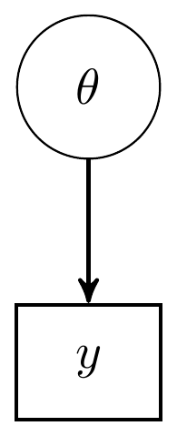
Figure 2.1: Directed Acyclic Graph (DAG) for the beta-binomial model
I have given an alternative DAG representation that includes all relevant details. In terms of a DAG, I prefer this representation as all the assumed model components are made explicit. However, in more complex models this approach will likely lead to very dense and possible unuseful representations.
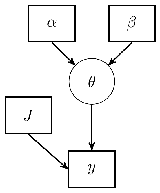
Figure 2.2: DAG with explicit representation for all beta-binomial model components
Yet another alternative representation is what I call a model specification chart. This takes on a similar feel as a DAG in that the flow of model parameters can be shown, but with the major difference that I use the distributional notation explicitly.
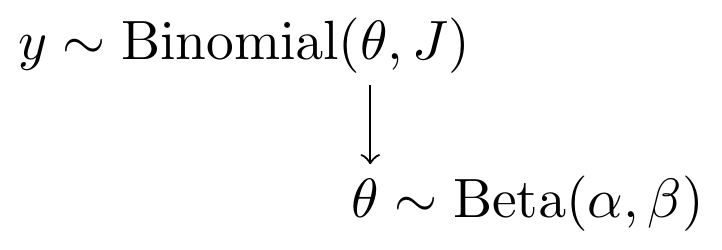
Figure 2.3: Model specification diagram for beta-binomial model
I will stick with these last two representations as much as possible.
2.1.1 Computation using Stan
Now, I’m finally getting to the analysis part.
I have done my best to be descriptive of what the Stan code represents and how it works (in a general how to use this sense).
I highly recommend a look at the example analysis by the development team to help see their approach as well (see here Stan analysis).
model_beta_binomial <- '
// data block needs to describe the variable
//  type (e.g., real, int, etc.) and the name
//  in the data object passed
data {
  int J;
  int y;
  real alpha;
  real beta;
}
// parameters block needs to specify the
//  unknown parameters
parameters {
  real<lower=0, upper=1>theta;
}
// model block needs to describe the data-model
//  and the prior specification
model {
  y ~ binomial(J, theta);
  theta ~ beta(alpha, beta);
}
// there must be a blank line after all blocks

'
# data must be in a list
mydata <- list(
  J = 10,
  y = 7,
  alpha = 6,
  beta = 6
)

# start values can be done automatically by stan or
#   done explicitly be the analyst (me). I prefer
#   to try to be explicit so that I can *try* to
#   guarantee that the initial chains start.
#   The values can be specified as a function
#   which lists the values to the respective
#   parameters
start_values <- function(){
  list(theta = 0.5)
}

# Next, need to fit the model
#   I have explicited outlined some common parameters
fit <- stan(
  model_code = model_beta_binomial, # model code to be compiled
  data = mydata,          # my data
  init = start_values,    # starting values
  chains = 4,             # number of Markov chains
  warmup = 1000,          # number of warmup iterations per chain
  iter = 2000,            # total number of iterations per chain
  cores = 2,              # number of cores (could use one per chain)
  refresh = 0             # no progress shown
)

# first get a basic breakdown of the posteriors
print(fit, pars="theta")
## Inference for Stan model: anon_model.
## 4 chains, each with iter=2000; warmup=1000; thin=1;
## post-warmup draws per chain=1000, total post-warmup draws=4000.
##
## mean se_mean sd 2.5% 25% 50% 75% 97.5% n_eff Rhat
## theta 0.59 0 0.1 0.39 0.53 0.6 0.66 0.78 1511 1
##
## Samples were drawn using NUTS(diag_e) at Sun Jun 19 17:27:45 2022.
## For each parameter, n_eff is a crude measure of effective sample size,
## and Rhat is the potential scale reduction factor on split chains (at
## convergence, Rhat=1).
# plot the posterior in a
#  95% probability interval
#  and 80% to contrast the dispersion
plot(fit, pars="theta")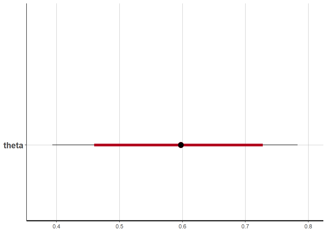
# plot the posterior density
posterior <- as.matrix(fit)

plot_title <- ggtitle("Posterior distributions",
                      "with medians and 80% intervals")
mcmc_areas(
  posterior,
  pars = c("theta"),
  prob = 0.8) +
  plot_title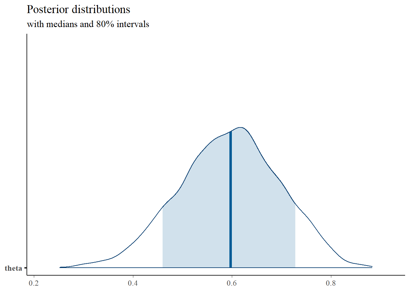
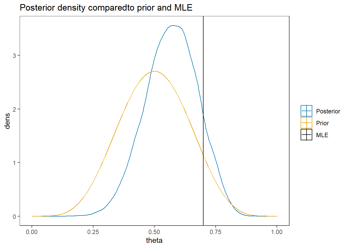
# I prefer a posterior plot that includes prior and MLE
MLE <- 0.7
prior <- function(x){dbeta(x, 6, 6)}
x <- seq(0, 1, 0.01)
prior.dat <- data.frame(X=x, dens = prior(x))
cols <- c("Posterior"="#0072B2", "Prior"="#E69F00", "MLE"= "black")#"#56B4E9", "#E69F00" "#CC79A7"
ggplot()+
  geom_density(data=as.data.frame(posterior),
               aes(x=theta, color="Posterior"))+
  geom_line(data=prior.dat,
            aes(x=x, y=dens, color="Prior"))+
  geom_vline(aes(xintercept=MLE, color="MLE"))+
  scale_color_manual(values=cols, name=NULL)+
  theme_bw()+
  theme(panel.grid = element_blank())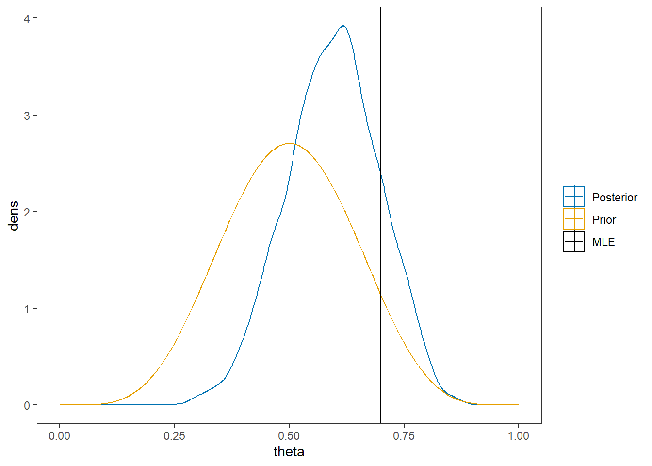
2.1.2 Computation using WinBUGS (OpenBUGS)
Here, I am simply contrasting the computation from Stan to how BPM describes the computations using WinBUGS. I have downloaded the .bug file from the text website and I will load it into R for viewing.
First, let’s take a look at the model described by BPM on p. 39.
# A model block
model{
  #################################
  # Prior distribution
  #################################
  theta ~ dbeta(alpha,beta)
  #################################
  # Conditional distribution of the data
  #################################
  y ~ dbin(theta, J)
}
# data statement
list(J = 10, y = 7, alpha = 6, beta = 6)
Next, we want to use the above model.
Using OpensBUGS through R can be a little clunky as I had to create objects with the filepaths of the data and model code then get R to read those in through the function openbugs.
Otherwise, the code is similar to style to the code used for calling Stan.
# model code
model.file <- paste0(w.d,"/code/Binomial/Binomial Model.bug")

# get data file
data.file <- paste0(w.d,"/code/Binomial/Binomial data.txt")

# starting values
start_values <- function(){
  list(theta=0.5)
}

# vector of all parameters to save
param_save <- c("theta")

# fit model
fit <- openbugs(
  data= data.file,
  model.file = model.file, # R grabs the file and runs it in openBUGS
  parameters.to.save = param_save,
  inits=start_values,
  n.chains = 4,
  n.iter = 2000,
  n.burnin = 1000,
  n.thin = 1
)

print(fit)

posterior <- fit$sims.matrix

plot_title <- ggtitle("Posterior distributions",
                      "with medians and 80% intervals")
mcmc_areas(
  posterior,
  pars = c("theta"),
  prob = 0.8) +
  plot_title


MLE <- 0.7
prior <- function(x){dbeta(x, 6, 6)}
x <- seq(0, 1, 0.01)
prior.dat <- data.frame(X=x, dens = prior(x))
cols <- c("Posterior"="#0072B2", "Prior"="#E69F00", "MLE"= "black")#"#56B4E9", "#E69F00" "#CC79A7"
ggplot()+
  geom_density(data=as.data.frame(posterior),
               aes(x=theta, color="Posterior"))+
  geom_line(data=prior.dat,
            aes(x=x, y=dens, color="Prior"))+
  geom_vline(aes(xintercept=MLE, color="MLE"))+
  labs(title="Posterior density comparedto prior and MLE")+
  scale_color_manual(values=cols, name=NULL)+
  theme_bw()+
  theme(panel.grid = element_blank())
2.1.3 Computation using JAGS (R2jags)
Here, I utilize JAGS, which is nearly identical to WinBUGS in how the underlying mechanics work to compute the posterior but is easily to use through R.
# model code
jags.model <- function(){
  #################################
  # Conditional distribution of the data
  #################################
  y ~ dbin(theta, J)
  #################################
  # Prior distribution
  #################################
  theta ~ dbeta(alpha, beta)
}
# data
mydata <- list(
  J = 10,
  y = 7,
  alpha = 6,
  beta = 6
)
# starting values
start_values <- function(){
  list("theta"=0.5)
}

# vector of all parameters to save
param_save <- c("theta")

# fit model
fit <- jags(
  model.file=jags.model,
  data=mydata,
  inits=start_values,
  parameters.to.save = param_save,
  n.iter=1000,
  n.burnin = 500,
  n.chains = 4,
  n.thin=1,
  progress.bar = "none")
## Compiling model graph
## Resolving undeclared variables
## Allocating nodes
## Graph information:
## Observed stochastic nodes: 1
## Unobserved stochastic nodes: 1
## Total graph size: 5
##
## Initializing model
print(fit)## Inference for Bugs model at "C:/Users/noahp/AppData/Local/Temp/RtmpQR8sbs/model45447f3b5e11.txt", fit using jags,
## 4 chains, each with 1000 iterations (first 500 discarded)
## n.sims = 2000 iterations saved
## mu.vect sd.vect 2.5% 25% 50% 75% 97.5% Rhat n.eff
## theta 0.596 0.103 0.396 0.525 0.596 0.670 0.791 1.002 2000
## deviance 3.536 1.056 2.644 2.749 3.151 3.937 6.416 1.004 960
##
## For each parameter, n.eff is a crude measure of effective sample size,
## and Rhat is the potential scale reduction factor (at convergence, Rhat=1).
##
## DIC info (using the rule, pD = var(deviance)/2)
## pD = 0.6 and DIC = 4.1
## DIC is an estimate of expected predictive error (lower deviance is better).
# extract posteriors for all chains
jags.mcmc <- as.mcmc(fit)
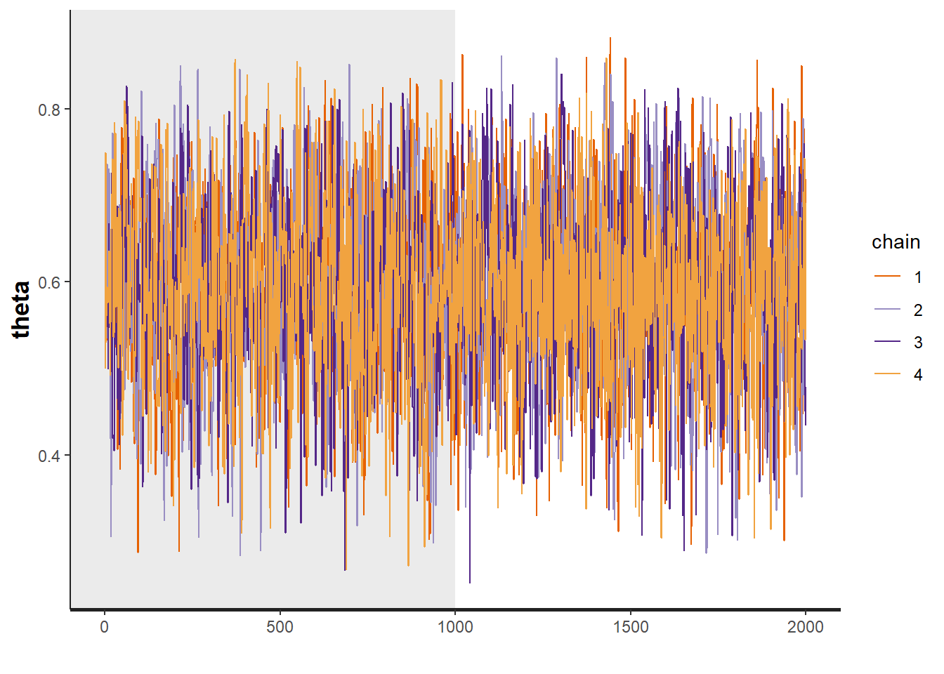
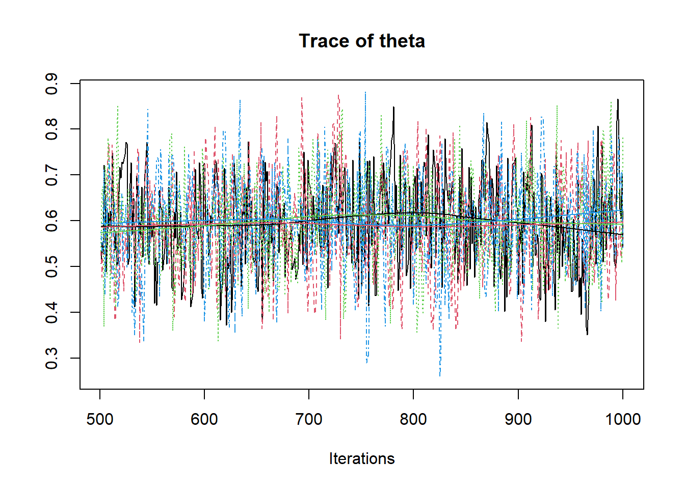
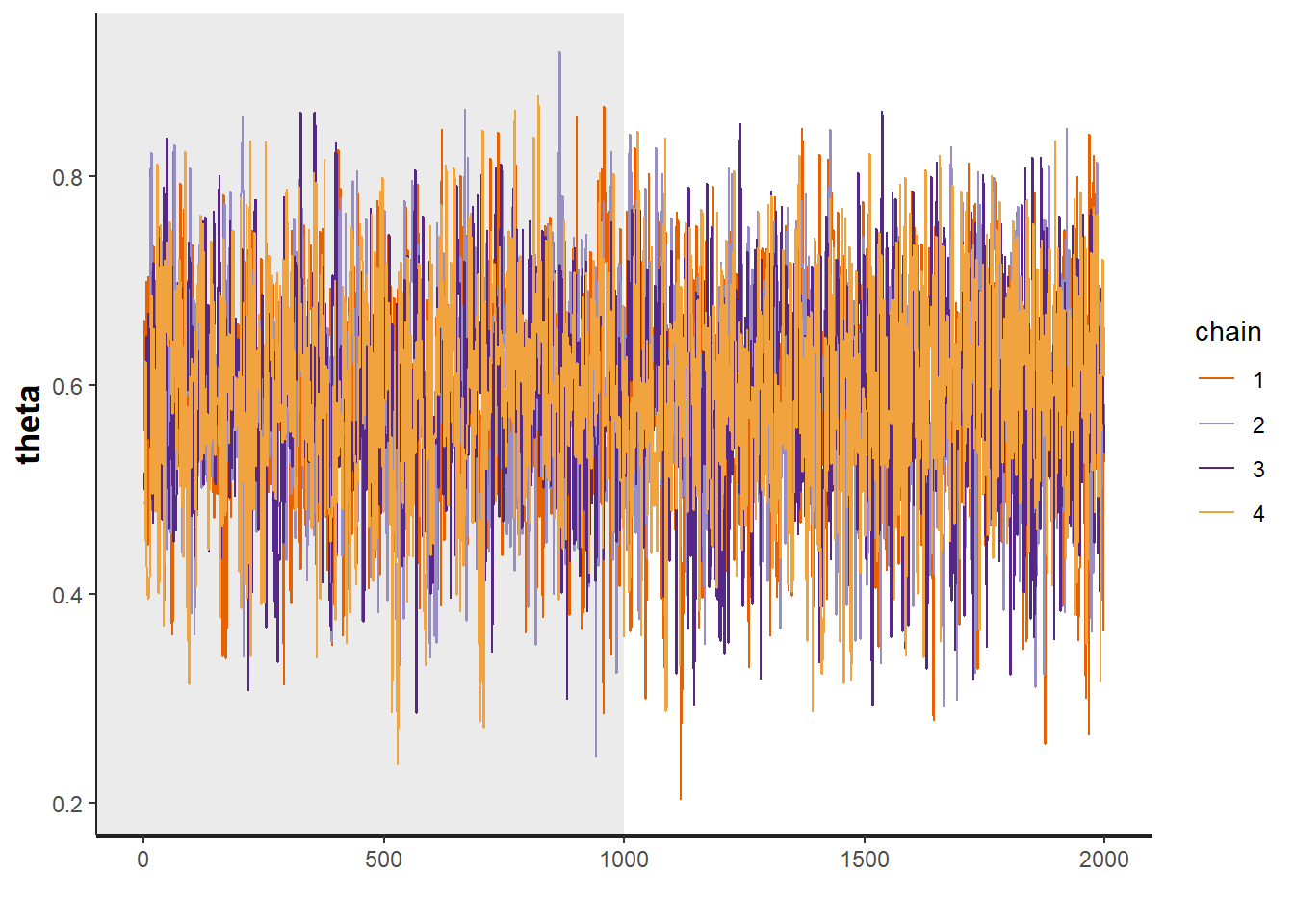
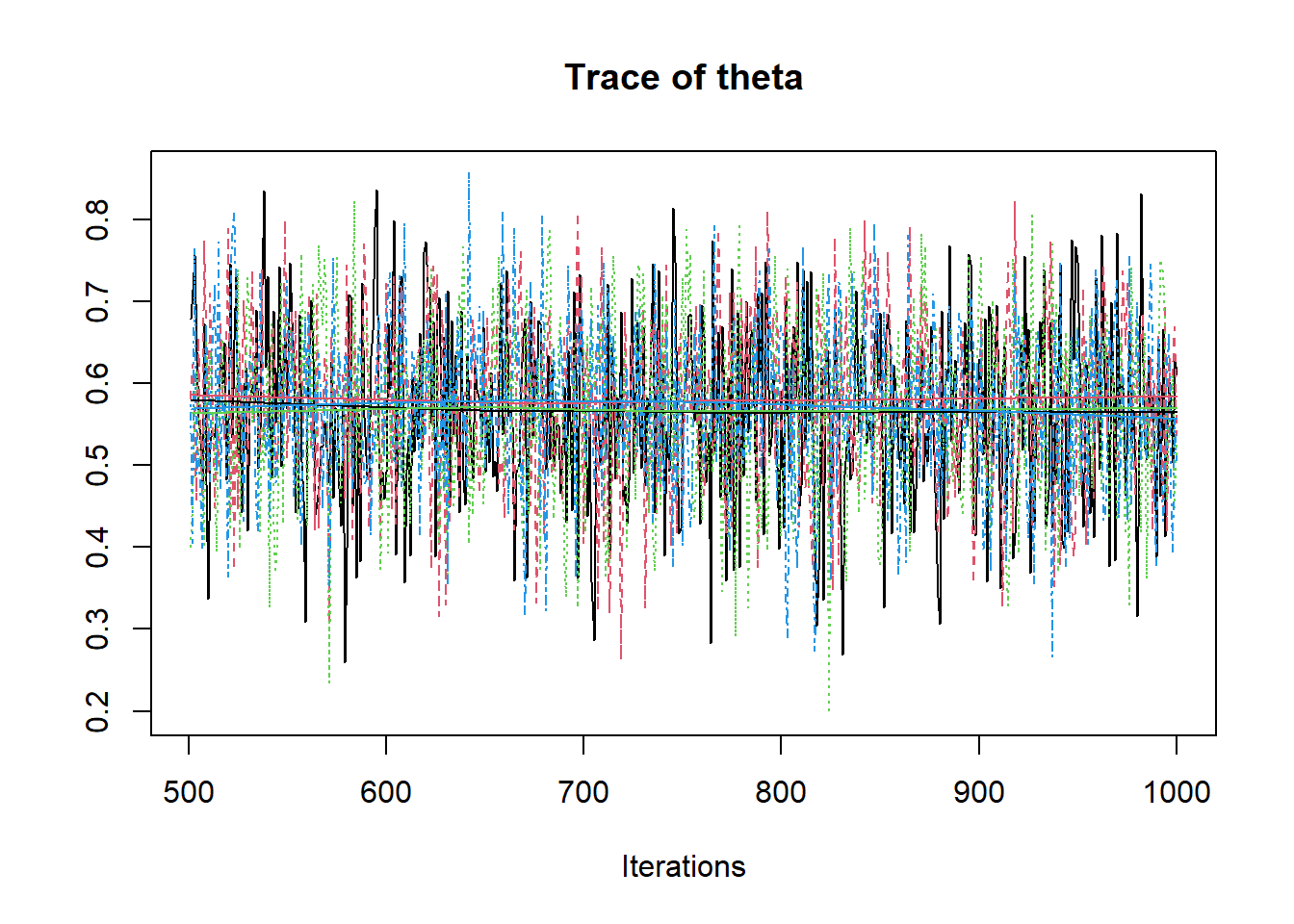
R2jags::traceplot(jags.mcmc)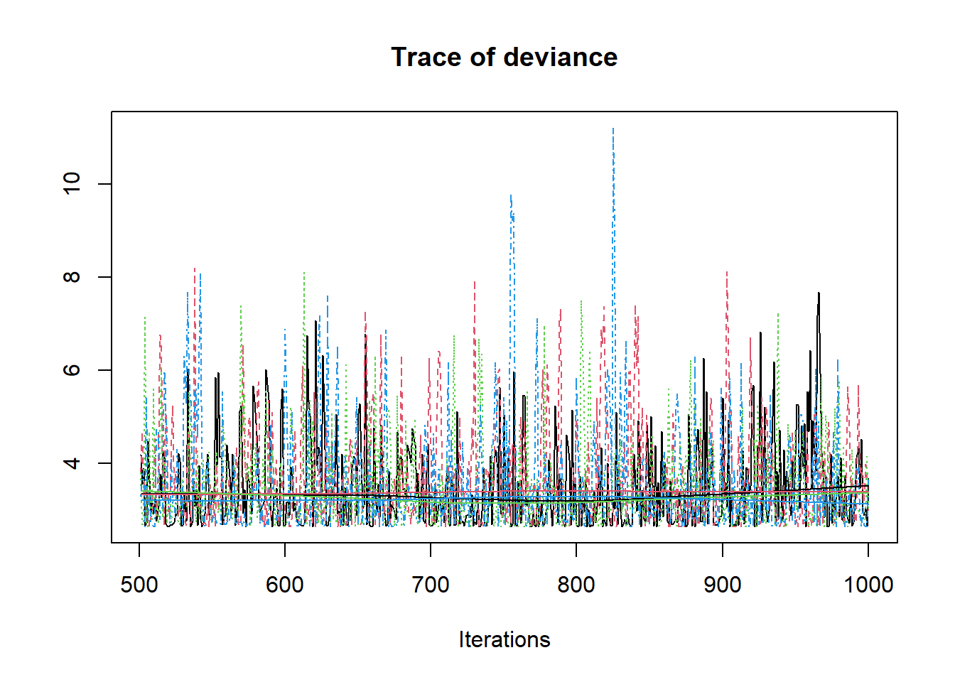
# convert to singel data.frame for density plot
a <- colnames(as.data.frame(jags.mcmc[[1]]))
plot.data <- data.frame(as.matrix(jags.mcmc, chains=T, iters = T))
colnames(plot.data) <- c("chain", "iter", a)


plot_title <- ggtitle("Posterior distributions",
                      "with medians and 80% intervals")
mcmc_areas(
  plot.data,
  pars = c("theta"),
  prob = 0.8) +
  plot_title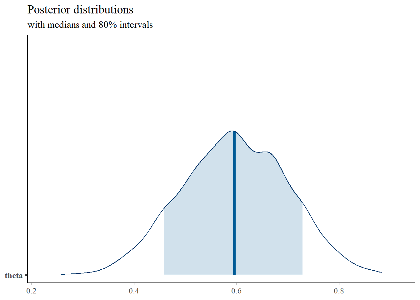
MLE <- 0.7
prior <- function(x){dbeta(x, 6, 6)}
x <- seq(0, 1, 0.01)
prior.dat <- data.frame(X=x, dens = prior(x))
cols <- c("Posterior"="#0072B2", "Prior"="#E69F00", "MLE"= "black")#"#56B4E9", "#E69F00" "#CC79A7"
ggplot()+
  geom_density(data=plot.data,
               aes(x=theta, color="Posterior"))+
  geom_line(data=prior.dat,
            aes(x=x, y=dens, color="Prior"))+
  geom_vline(aes(xintercept=MLE, color="MLE"))+
  labs(title="Posterior density comparedto prior and MLE")+
  scale_color_manual(values=cols, name=NULL)+
  theme_bw()+
  theme(panel.grid = element_blank())
2.2 Beta-Bernoulli Example
For this next example, I use the same data as the previous model. But now, instead of treating the individual events as part of a whole and sum over the successes, I will treat the model in a more hierarchical manner. A hierarchical model here simply implies that I’ll be using the same probability function for all individual observations. We express this by saying that the observations depend on the index (\(j=1, 2, ..., J\)) but that the parameter of interest does not vary across \(j\). Two DAG representations similar to the previous examples are shown below. The major difference in these representations from the previous example is the inclusion of a plate that represents the observations depend on the index \(j\).
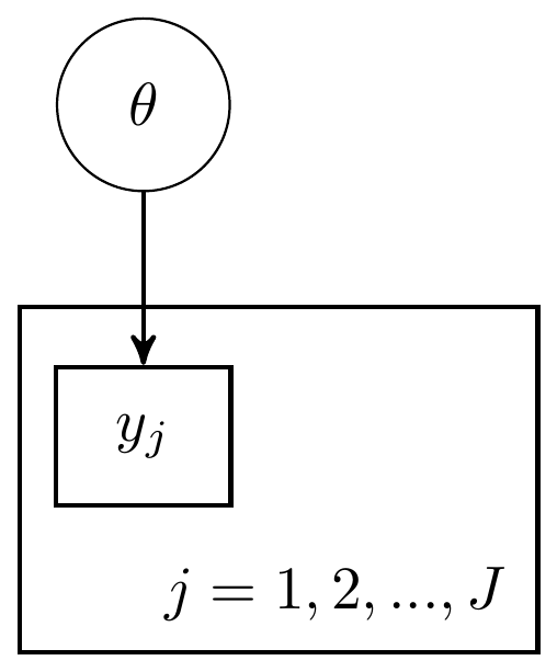
Figure 2.4: DAG for the beta-bernoulli model
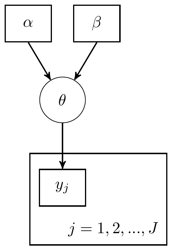
Figure 2.5: DAG with explicit representation for all beta-bernoulli model components
In my flavor of representation, this model can be expressed as
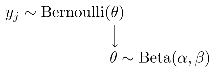
Figure 2.6: Model specification diagram for beta-bernoulli model
We will use the same \(\mathrm{Beta}(\alpha, \beta)\) prior for \(\theta\) as in the previous example. The model code changes to the following,
2.2.1 Computation using Stan
model_beta_bernoulli <- '
// data block needs to describe the variable
//  type (e.g., real, int, etc.) and the name
//  in the data object passed
data {
  int J;
  int y[J];  //declare observations as an integer vector of length J
  real alpha;
  real beta;
}
// parameters block needs to specify the
//  unknown parameters
parameters {
  real<lower=0, upper=1>theta;
}
// model block needs to describe the data-model
//  and the prior specification
model {
  for(j in 1:J){
    y[j] ~ bernoulli(theta);
  }
  theta ~ beta(alpha, beta);
}
// there must be a blank line after all blocks

'
# data must be in a list
mydata <- list(
  J = 10,
  y = c(1,0,1,1,0,0,1,1,1,1),
  alpha = 6,
  beta = 6
)

# start values can be done automatically by stan or
#   done explicitly be the analyst (me). I prefer
#   to try to be explicit so that I can *try* to
#   guarantee that the initial chains start.
#   The values can be specified as a function
#   which lists the values to the respective
#   parameters
start_values <- function(){
  list(theta = 0.5)
}

# Next, need to fit the model
#   I have explicited outlined some common parameters
fit <- stan(
  model_code = model_beta_bernoulli, # model code to be compiled
  data = mydata,          # my data
  init = start_values,    # starting values
  chains = 4,             # number of Markov chains
  warmup = 1000,          # number of warmup iterations per chain
  iter = 2000,            # total number of iterations per chain
  cores = 2,              # number of cores (could use one per chain)
  refresh = 0             # no progress shown
)

# first get a basic breakdown of the posteriors
print(fit, pars="theta")
## Inference for Stan model: anon_model.
## 4 chains, each with iter=2000; warmup=1000; thin=1;
## post-warmup draws per chain=1000, total post-warmup draws=4000.
##
## mean se_mean sd 2.5% 25% 50% 75% 97.5% n_eff Rhat
## theta 0.59 0 0.1 0.38 0.53 0.6 0.67 0.78 1527 1
##
## Samples were drawn using NUTS(diag_e) at Sun Jun 19 17:28:34 2022.
## For each parameter, n_eff is a crude measure of effective sample size,
## and Rhat is the potential scale reduction factor on split chains (at
## convergence, Rhat=1).
# plot the posterior in a
#  95% probability interval
#  and 80% to contrast the dispersion
plot(fit, pars="theta")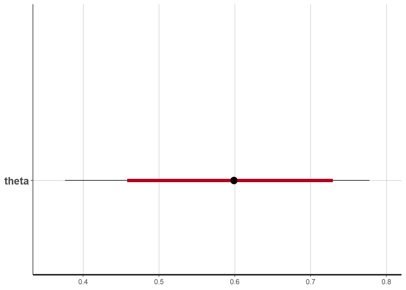
# plot the posterior density
posterior <- as.matrix(fit)

plot_title <- ggtitle("Posterior distributions",
                      "with medians and 80% intervals")
mcmc_areas(
  posterior,
  pars = c("theta"),
  prob = 0.8) +
  plot_title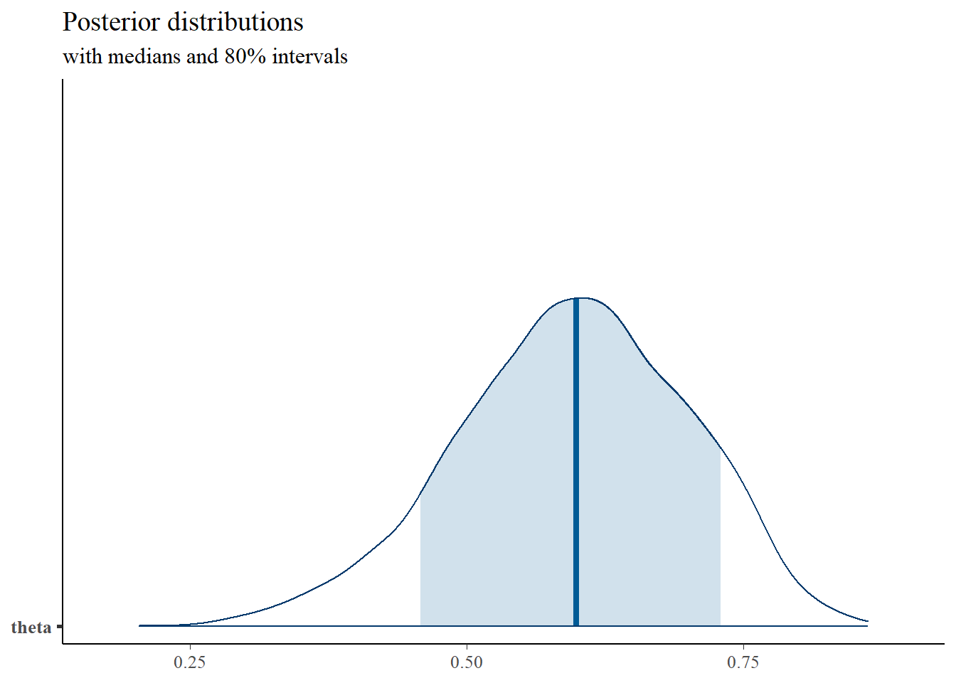
# I prefer a posterior plot that includes prior and MLE
MLE <- 0.7
prior <- function(x){dbeta(x, 6, 6)}
x <- seq(0, 1, 0.01)
prior.dat <- data.frame(X=x, dens = prior(x))
cols <- c("Posterior"="#0072B2", "Prior"="#E69F00", "MLE"= "black")#"#56B4E9", "#E69F00" "#CC79A7"
ggplot()+
  geom_density(data=as.data.frame(posterior),
               aes(x=theta, color="Posterior"))+
  geom_line(data=prior.dat,
            aes(x=x, y=dens, color="Prior"))+
  geom_vline(aes(xintercept=MLE, color="MLE"))+
  scale_color_manual(values=cols, name=NULL)+
  theme_bw()+
  theme(panel.grid = element_blank())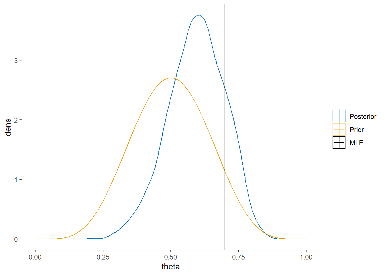
2.2.2 Computation using WinBUGS (OpenBUGS)
Here, I am simply contrasting the computation from Stan to how BPM describes the computations using WinBUGS. First, let’s take a look at the model described by BPM on p. 41.
# A model block
model{
  #################################
  # Prior distribution
  #################################
  theta ~ dbeta(alpha,beta)

  #################################
  # Conditional distribution of the data
  #################################
  for(j in 1:J){
    y[j] ~ dbern(theta)
  }
}
# data statement
list(J=10, y=c(1,0,1,0,1,1,1,1,0,1), alpha=6, beta=6)
The code is similar to style to the code used for calling Stan. However you’ll notice a difference in how a probability distribution is referenced.
# model code
model.file <- paste0(w.d,"/code/Bernoulli/Bernoulli Model.bug")

# get data file
data.file <- paste0(w.d,"/code/Bernoulli/Bernoulli data.txt")

# starting values
start_values <- function(){
  list(theta=0.5)
}

# vector of all parameters to save
param_save <- c("theta")

# fit model
fit <- openbugs(
  data= data.file,
  model.file = model.file, # R grabs the file and runs it in openBUGS
  parameters.to.save = param_save,
  inits=start_values,
  n.chains = 4,
  n.iter = 2000,
  n.burnin = 1000,
  n.thin = 1
)

print(fit)

posterior <- fit$sims.matrix

plot_title <- ggtitle("Posterior distributions",
                      "with medians and 80% intervals")
mcmc_areas(
  posterior,
  pars = c("theta"),
  prob = 0.8) +
  plot_title


MLE <- 0.7
prior <- function(x){dbeta(x, 6, 6)}
x <- seq(0, 1, 0.01)
prior.dat <- data.frame(X=x, dens = prior(x))
cols <- c("Posterior"="#0072B2", "Prior"="#E69F00", "MLE"= "black")#"#56B4E9", "#E69F00" "#CC79A7"
ggplot()+
  geom_density(data=as.data.frame(posterior),
               aes(x=theta, color="Posterior"))+
  geom_line(data=prior.dat,
            aes(x=x, y=dens, color="Prior"))+
  geom_vline(aes(xintercept=MLE, color="MLE"))+
  labs(title="Posterior density comparedto prior and MLE")+
  scale_color_manual(values=cols, name=NULL)+
  theme_bw()+
  theme(panel.grid = element_blank())
2.2.3 Computation using JAGS (R2jags)
Here, I utilize JAGS, which is nearly identical to WinBUGS in how the underlying mechanics work to compute the posterior but is easily to use through R.
# model code
jags.model <- function(){
  #################################
  # Conditional distribution of the data
  #################################
  for(j in 1:J){
    y[j] ~ dbern(theta)
  }

  #################################
  # Prior distribution
  #################################
  theta ~ dbeta(alpha,beta)

}
# data
mydata <- list(
  J = 10,
  y = c(1,0,1,1,0,0,1,NA,1,1),
  alpha = 6,
  beta = 6
)

# starting values
start_values <- function(){
  list("theta"=0.5)
}

# vector of all parameters to save
param_save <- c("theta")

# fit model
fit <- jags(
  model.file=jags.model,
  data=mydata,
  inits=start_values,
  parameters.to.save = param_save,
  n.iter=1000,
  n.burnin = 500,
  n.chains = 4,
  n.thin=1,
  progress.bar = "none")
## Compiling model graph
## Resolving undeclared variables
## Allocating nodes
## Graph information:
## Observed stochastic nodes: 9
## Unobserved stochastic nodes: 2
## Total graph size: 14
##
## Initializing model
print(fit)## Inference for Bugs model at "C:/Users/noahp/AppData/Local/Temp/RtmpQR8sbs/model454429615b74.txt", fit using jags,
## 4 chains, each with 1000 iterations (first 500 discarded)
## n.sims = 2000 iterations saved
## mu.vect sd.vect 2.5% 25% 50% 75% 97.5% Rhat n.eff
## theta 0.570 0.105 0.359 0.498 0.572 0.644 0.764 1.003 1200
## deviance 12.223 0.991 11.458 11.548 11.849 12.511 14.968 1.005 700
##
## For each parameter, n.eff is a crude measure of effective sample size,
## and Rhat is the potential scale reduction factor (at convergence, Rhat=1).
##
## DIC info (using the rule, pD = var(deviance)/2)
## pD = 0.5 and DIC = 12.7
## DIC is an estimate of expected predictive error (lower deviance is better).
# extract posteriors for all chains
jags.mcmc <- as.mcmc(fit)

R2jags::traceplot(jags.mcmc)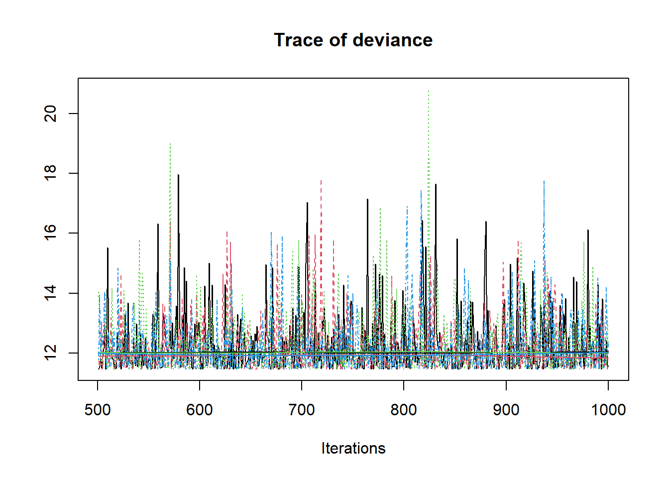
# convert to singel data.frame for density plot
a <- colnames(as.data.frame(jags.mcmc[[1]]))
plot.data <- data.frame(as.matrix(jags.mcmc, chains=T, iters = T))
colnames(plot.data) <- c("chain", "iter", a)


plot_title <- ggtitle("Posterior distributions",
                      "with medians and 80% intervals")
mcmc_areas(
  plot.data,
  pars = c("theta"),
  prob = 0.8) +
  plot_title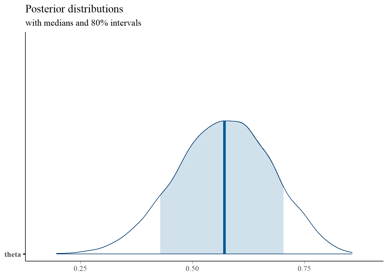
MLE <- 0.7
prior <- function(x){dbeta(x, 6, 6)}
x <- seq(0, 1, 0.01)
prior.dat <- data.frame(X=x, dens = prior(x))
cols <- c("Posterior"="#0072B2", "Prior"="#E69F00", "MLE"= "black")#"#56B4E9", "#E69F00" "#CC79A7"
ggplot()+
  geom_density(data=plot.data,
               aes(x=theta, color="Posterior"))+
  geom_line(data=prior.dat,
            aes(x=x, y=dens, color="Prior"))+
  geom_vline(aes(xintercept=MLE, color="MLE"))+
  labs(title="Posterior density comparedto prior and MLE")+
  scale_color_manual(values=cols, name=NULL)+
  theme_bw()+
  theme(panel.grid = element_blank())