11 Item Response Theory

Item response theory (IRT) builds models for item (stimuli that the measures collected) based on two broad classes of models

1. Models for dichotomous (binary, 0/1) items and
2. Models for polytomous (multi-category) items.

11.1 IRT Models for Dichotomous Data

First, for conventional dichotomous observed variables, an IRT model can be generally specified as follows.

Let \(x_{ij}\) be the observed value from respondent \(i\) on observable (item) \(j\). When \(x\) is binary, the observed value can be \(0\) or \(1\). Some common IRT models for binary observed variables can be expressed as a version of

\[p(x_{ij} = 1 \mid \theta_i, d_j, a_j, c_j) = c_j + (1-c_j)F(a_j \theta_i + d_j),\]

where,

• \(\theta_i\) is the magnitude of the latent variable that individual \(i\) possesses. In educational measurement, \(\theta_i\) commonly represents proficiency so that a higher \(\theta_i\) means that individual has more of the trait,
• \(d_j\) is the item location or difficulty parameter. \(d_j\) is commonly transformed to be \(d_j = -a_jb_j\) so that the location parameter is easier to interpret in relation to the latent trait \(\theta_i\),
• \(a_j\) is the item slope or discrimination parameter,
• \(c_j\) is the item lower asymptote or guessing parameter,
• \(F(.)\) is the link function to be specified that determines the form of the transformation between latent trait and the item response probability. The link is common chosen to be either the logistic link or the normal-ogive link.

Common IRT models are the

• 1-PL, or one-parameter logistic model, which only uses one measurement parameter \(d_j\) per item,
• 2-PL, or two-parameter logistic model, which uses two measurement model parameters \(a_j\) and \(d_j\) per item,
• 3-PL, or three-parameter logistic model, which uses all three parameters as shown above.
• other models are also possible for binary item response formats but are omitted here.

The above describes the functional form used to model why individual may have a greater or lesser likelihood of endorsing an item (have a \(1\) as a measure). We use the above model as the basis for defining the conditional probability of any response given the values of the parameters. The conditional probability is then commonly used as part of a marginal maximum likelihood (MML) approach to finding parameters values for the measurement model which maximize the likelihood. However, given that the values of the latent variable \(\theta_i\) are also unknown, the distribution of \(\theta_i\) is marginalized out of the likelihood function.

However, in the Bayesian formulation, we can side-step some of these issues by the use of prior distributions. Starting with the general form of the likelihood function \[p(\mathbf{x}\mid \boldsymbol{\theta}, \boldsymbol{\omega}) = \prod_{i=1}^np(\mathbf{x}_i\mid \theta_i, \boldsymbol{\omega}) = \prod_{i=1}^n\prod_{j=1}^Jp(x_{ij}\mid \theta_i, \boldsymbol{\omega}_j),\] where \[x_{ij}\mid \theta_i, \boldsymbol{\omega}_j \sim \mathrm{Bernoulli}[p(x_{ij}\mid \theta_i, \boldsymbol{\omega}_j)].\]

Developing a joint prior distribution for \(p(\boldsymbol{\theta}, \boldsymbol{\omega})\) is not straightforward given the high dimensional aspect of the components. But, a common assumption is that the distribution for the latent variables (\(\boldsymbol{\theta}\)) is independent of the distribution for the measurement model parameters (\(\boldsymbol{\omega}\)). That is, we can separate the problem into independent priors \[p(\boldsymbol{\theta}, \boldsymbol{\omega}) = p(\boldsymbol{\theta})p(\boldsymbol{\omega}).\]

For the latent variables, the prior distributuion is generally build by assuming that all individuals are also independent. The independence of observations leads to a joint prior that is a product of priors with a common distribution, \[p(\boldsymbol{\theta}) = \prod_{i=1}^np(\theta_i\mid \boldsymbol{\theta}_p),\] where \(\boldsymbol{\theta}_p\) are the hyperparameters governing the common prior for the latent variable distribution. A common choice is that \(\theta_i \sim \mathrm{Normal}(\mu_{\theta} = 0, \sigma^2_{\theta}=1)\) because the distribution is arbitrary.

For the measurement model parameters, a bit more complex specification is generally needed. One simple approach would be to invoke an exchangeability assumption among items and among item parameters. This would essentially make all priors independent and simplify the specification to product of univariate priors over all measurement model parameters \[p(\boldsymbol{\omega}) = \prod_{j=1}^Jp(\boldsymbol{\omega}_j)=\prod_{j=1}^Jp(d_j)p(a_j)p(c_j).\] For for location parameter (\(d_j\)), a common prior distribution is an unbounded normal distribution. Because, the location can take on any value within the range of the latent variable which is also technically unbounded so we let \[d_j \sim \mathrm{Normal}(\mu_{d},\sigma^2_d).\] The choice of hyperparameters can be guided by prior research or set to a common relative diffuse value for all items such as \(\mu_{d}=0,\sigma^2_d=10\).

The discrimination parameter governs the strength of the relationship between the latent variable and the probability of endorsing the item. This is similar in flavor to a factor loading in CFA. An issue with specifying a prior for the discrimination parameter is the indeterminacy with respect the the orientation of the latent variable. In CFA, we resolved the orientation indeterminacy issue by fixing one factor loading to 1. In IRT, we can do so by constraining the possible values of the discrimination parameters to be strictly positive. This forces each item to have the meaning of higher values on the latent variable directly (or at least proportionally) increase the probability of endorsing the item. We achieve this by using a prior such as \[a_j \sim \mathrm{Normal}^{+}(\mu_a,\sigma^2_a).\] The term \(\mathrm{Normal}^{+}(.)\) means that the normal distribution is truncated at 0 so that only positive values are possible.

Lastly, the guessing parameter \(c_j\) takes on values between \([0,1]\). A common choice for parameters bounded between 0 and 1 is a Beta prior, that is \[c_j \sim \mathrm{Beta}(\alpha_c, \beta_c).\] The hyperparameters \(\alpha_c\) and \(\beta_c\) determine the shape of the beta prior and affect the likelihood and magnitude of guessing parameters.

11.2 3-PL LSAT Example

In the Law School Admission Test (LSAT) example (p. 263-271), the data are from 1000 examinees responding to five items which is just a subset of the LSAT. We hypothesize that only one underlying latent variable is measured by these items. But that guessing is also plausible. The full 3-PL model we will use can be described in an equation as \[p(\boldsymbol{\theta}, \boldsymbol{d}, \boldsymbol{a}, \boldsymbol{c} \mid \mathbf{x}) \propto \prod_{i=1}^n\prod_{j=1}^Jp(\theta_i\mid\theta_i, d_j, a_j, c_j)p(\theta_i)p(d_j)p(a_j)p(c_j),\] where \[\begin{align*} x_{ij}\mid\theta_i\mid\theta_i, d_j, a_j, c_j &\sim \mathrm{Bernoulli}[p(\theta_i\mid\theta_i, d_j, a_j, c_j)],\ \mathrm{for}\ i=1, \cdots, 100,\ j = 1, \cdots, 5;\\ p(\theta_i\mid\theta_i, d_j, a_j, c_j) &= c_j + (1-c_j)\Phi(a_j\theta_j + d_j),\ \mathrm{for}\ i=1, \cdots, 100,\ j = 1, \cdots, 5;\\ \theta_i &\sim \mathrm{Normal}(0,1),\ \mathrm{for}\ i = 1, \cdots, 1000;\\ d_j &\sim \mathrm{Normal}(0, 2),\ \mathrm{for}\ j=1, \cdots, 5;\\ a_j &\sim \mathrm{Normal}^{+}(1, 2),\ \mathrm{for}\ j=1, \cdots, 5;\\ c_j &\sim \mathrm{Beta}(5, 17),\ \mathrm{for}\ j=1, \cdots, 5. \end{align*}\]

The above model can illustrated in a DAG as shown below.

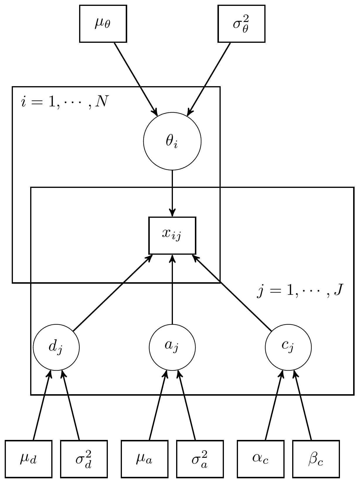
Figure 11.1: DAG for 3-PL IRT model for LSAT Example

The path diagram for an IRT is essentially identical to the path diagram for a CFA model. This fact highlights an important feature of IRT/CFA in that the major conceptual difference between these approaches to is how we define the link between the latent variable the observed items.

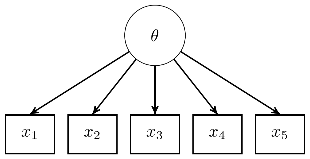
Figure 11.2: Path diagram for 3-PL IRT model

For completeness, I have included the model specification diagram that more concretely connects the DAG and path diagram to the assumed distributions and priors.

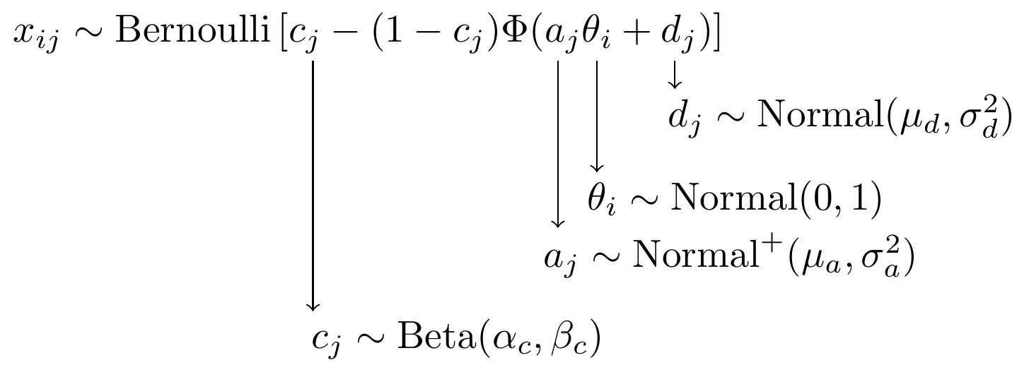
Figure 11.3: Model specification diagram for the 3-PL IRT model

11.3 LSAT Example - JAGS

jags.model.lsat <- function(){

#########################################
# Specify the item response measurement model for the observables
#########################################
for (i in 1:n){
  for(j in 1:J){
    P[i,j] <- c[j]+(1-c[j])*phi(a[j]*theta[i]+d[j])       # 3P-NO expression
    x[i,j] ~ dbern(P[i,j])                  # distribution for each observable
  }
}


##########################################
# Specify the (prior) distribution for the latent variables
##########################################
for (i in 1:n){
  theta[i] ~ dnorm(0, 1)  # distribution for the latent variables
}


##########################################
# Specify the prior distribution for the measurement model parameters
##########################################
for(j in 1:J){
  d[j] ~ dnorm(0, .5)          # Locations for observables
  a[j] ~ dnorm(1, .5); I(0,)    # Discriminations for observables
  c[j] ~ dbeta(5,17)           # Lower asymptotes for observables
  
}


} # closes the model

# initial values
start_values <- list(
  list("d"=c(1.00, 1.00, 1.00, 1.00, 1.00),
       "a"=c(1.00, 1.00, 1.00, 1.00, 1.00),
       "c"=c(0.20, 0.20, 0.20, 0.20, 0.20)),
  list("d"=c(-3.00, -3.00, -3.00, -3.00, -3.00),
       "a"=c(3.00, 3.00, 3.00, 3.00, 3.00),
       "c"=c(0.50, 0.50, 0.50, 0.50, 0.50)),
  list("d"=c(3.00, 3.00, 3.00, 3.00, 3.00),
       "a"=c(0.1, 0.1, 0.1, 0.1, 0.1),
       "c"=c(0.05, 0.05, 0.05, 0.05, 0.05))
)

# vector of all parameters to save
param_save <- c("a", "c", "d", "theta")

# dataset
dat <- read.table("data/LSAT.dat", header=T)

mydata <- list(
  n = nrow(dat), J = ncol(dat),
  x = as.matrix(dat)
)

# fit model
fit <- jags(
  model.file=jags.model.lsat,
  data=mydata,
  inits=start_values,
  parameters.to.save = param_save,
  n.iter=2000,
  n.burnin = 1000,
  n.chains = 3,
  progress.bar = "none")

## module glm loaded

## Compiling model graph
##    Resolving undeclared variables
##    Allocating nodes
## Graph information:
##    Observed stochastic nodes: 5000
##    Unobserved stochastic nodes: 1015
##    Total graph size: 31027
## 
## Initializing model

#print(fit)
round(fit$BUGSoutput$summary[ !rownames(fit$BUGSoutput$summary) %like% "theta", ], 3)

##              mean     sd     2.5%      25%      50%      75%    97.5%  Rhat n.eff
## a[1]        0.455  0.163    0.194    0.341    0.437    0.544    0.813 1.030    85
## a[2]        0.680  0.407    0.298    0.447    0.563    0.713    1.834 1.181    24
## a[3]        1.231  0.675    0.433    0.753    1.055    1.524    2.968 1.090    55
## a[4]        0.480  0.149    0.232    0.367    0.469    0.575    0.805 1.018   140
## a[5]        0.459  0.158    0.181    0.350    0.441    0.549    0.818 1.006   740
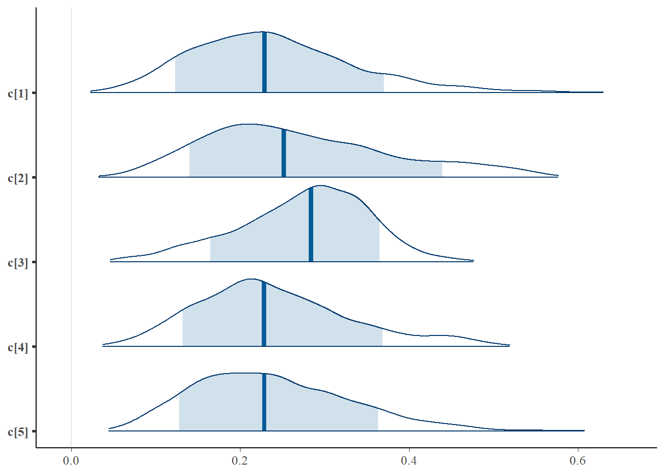
## c[1]        0.238  0.096    0.081    0.169    0.229    0.295    0.460 1.002  2300
## c[2]        0.270  0.111    0.097    0.187    0.252    0.340    0.515 1.120    24
## c[3]        0.275  0.077    0.108    0.227    0.284    0.330    0.407 1.023   100
## c[4]        0.240  0.091    0.091    0.176    0.228    0.294    0.454 1.001  3000
## c[5]        0.238  0.092    0.090    0.169    0.229    0.298    0.441 1.004  3000
## d[1]        1.408  0.135    1.130    1.325    1.409    1.487    1.693 1.010   320
## d[2]        0.243  0.267   -0.565    0.167    0.316    0.410    0.538 1.288    16
## d[3]       -0.563  0.405   -1.495   -0.778   -0.475   -0.277    0.016 1.098    30
## d[4]        0.530  0.134    0.186    0.466    0.548    0.620    0.741 1.001  3000
## d[5]        1.043  0.119    0.785    0.972    1.051    1.124    1.253 1.020   620
## deviance 4518.533 69.740 4362.905 4475.720 4523.581 4565.875 4645.075 1.082    35

# extract posteriors for all chains
jags.mcmc <- as.mcmc(fit)
# the below two plots are too big to be useful given the 1000 observations.
#R2jags::traceplot(jags.mcmc)

# gelman-rubin-brook
#gelman.plot(jags.mcmc)

# convert to single data.frame for density plot
a <- colnames(as.data.frame(jags.mcmc[[1]]))
plot.data <- data.frame(as.matrix(jags.mcmc, chains=T, iters = T))
colnames(plot.data) <- c("chain", "iter", a)


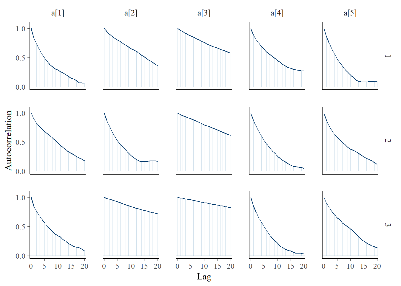
bayesplot::mcmc_acf(plot.data,pars = c(paste0("d[", 1:5, "]")))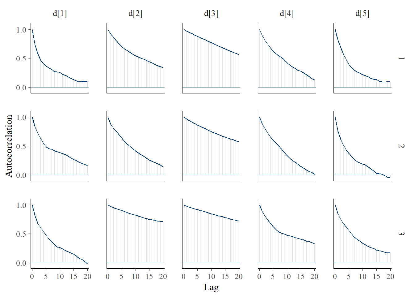

bayesplot::mcmc_trace(plot.data,pars = c(paste0("d[", 1:5, "]")))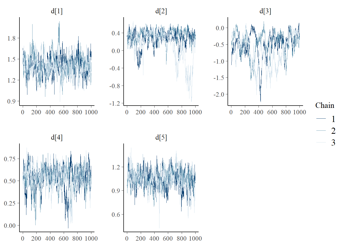

ggmcmc::ggs_grb(ggs(jags.mcmc), family="d")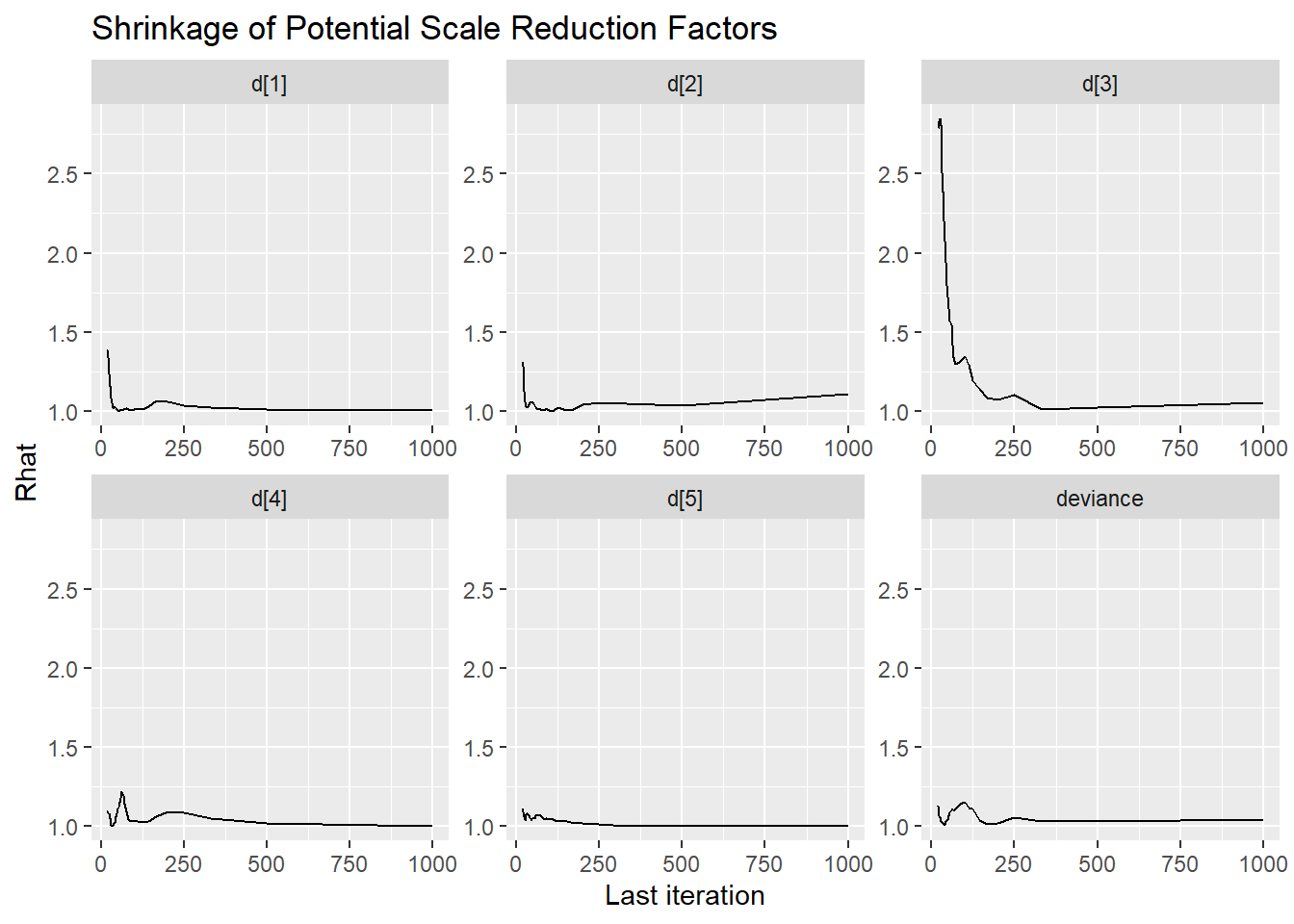

mcmc_areas(plot.data, pars = c(paste0("d[",1:5,"]")), prob = 0.8)

bayesplot::mcmc_acf(plot.data,pars = c(paste0("a[", 1:5, "]")))

bayesplot::mcmc_trace(plot.data,pars = c(paste0("a[", 1:5, "]")))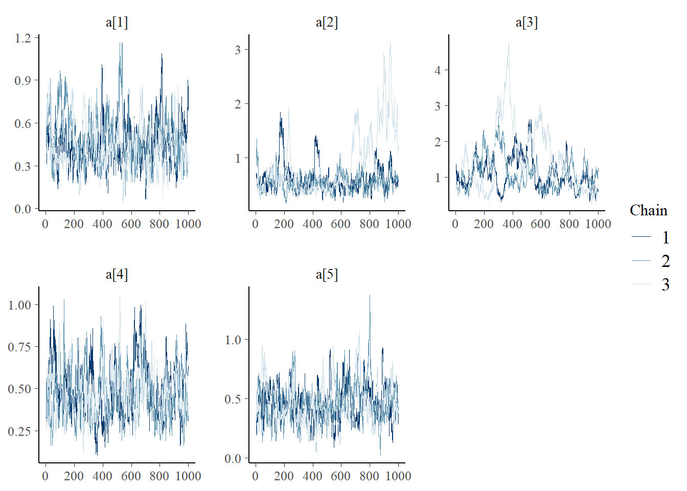

ggmcmc::ggs_grb(ggs(jags.mcmc), family="a")

mcmc_areas( plot.data,pars = c(paste0("a[", 1:5, "]")), prob = 0.8)

bayesplot::mcmc_acf(plot.data,pars = c(paste0("c[", 1:5, "]")))

bayesplot::mcmc_trace(plot.data,pars = c(paste0("c[", 1:5, "]")))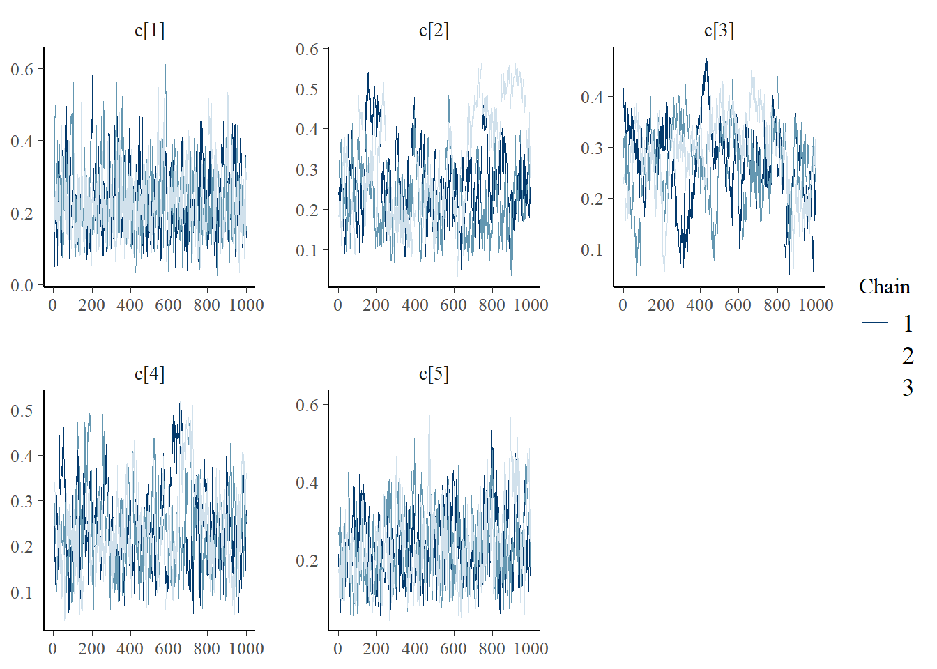

ggmcmc::ggs_grb(ggs(jags.mcmc), family="c")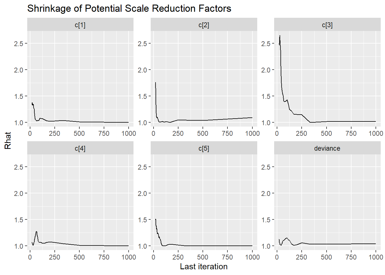

mcmc_areas(plot.data, pars = c(paste0("c[", 1:5, "]")), prob = 0.8)

11.3.1 Posterior Predicted Distributions

Here, we want to compare the observed and expected posterior predicted distributions.

Statistical functions of interest are the (1) standardized model-based covariance (SMBC) and (2) the standardized generalized discrepancy measure (SGDDM).

For (1), the SMBC is \[SMBC_{jj^\prime}=\frac{\frac{1}{n}\sum_{i=1}^n(x_{ij} - E(x_{ij} \mid \theta_i,\boldsymbol{\omega}_j))(x_{ij^\prime} - E(x_{ij^\prime} \mid \theta_i,\boldsymbol{\omega}_j^\prime))}{\sqrt{\frac{1}{n}\sum_{i=1}^n(x_{ij} - E(x_{ij} \mid \theta_i,\boldsymbol{\omega}_j))^2}\sqrt{\frac{1}{n}\sum_{i=1}^n(x_{ij^\prime} - E(x_{ij^\prime} \mid \theta_i,\boldsymbol{\omega}_j^\prime))}}\]

In R, the functions below can be used to compute these qualtities.

calculate.SGDDM <- function(data.matrix, expected.value.matrix){
    
    J.local = ncol(data.matrix)

    SMBC.matrix <- calculate.SMBC.matrix(data.matrix, expected.value.matrix)
    
    SGDDM = sum(abs((lower.tri(SMBC.matrix, diag=FALSE))*SMBC.matrix))/((J.local*(J.local-1))/2)

    SGDDM

} # closes calculate.SGDDM

calculate.SMBC.matrix <- function(data.matrix, expected.value.matrix){
    
    N.local <- nrow(data.matrix)

    MBC.matrix <- (t(data.matrix-expected.value.matrix) %*% (data.matrix-expected.value.matrix))/N.local

    MBStddevs.matrix <- diag(sqrt(diag(MBC.matrix)))

    #SMBC.matrix <- solve(MBStddevs.matrix) %*% MBC.matrix %*% solve(MBStddevs.matrix)


    J.local <- ncol(data.matrix)

    SMBC.matrix <- matrix(NA, nrow=J.local, ncol=J.local)

    for(j in 1:J.local){
        for(jj in 1:J.local){
            SMBC.matrix[j,jj] <- MBC.matrix[j,jj]/(MBStddevs.matrix[j,j]*MBStddevs.matrix[jj,jj])
        }
    }

    SMBC.matrix 

} # closes calculate.MBC.matrix

Next, we will use the functions above among other basic data wrangling to construct a full posterior predictive distribution analysis to probe our resulting posterior.

# Data wrangle the results/posterior draws for use
datv1 <- plot.data %>%
  pivot_longer(
    cols = `a[1]`:`a[5]`,
    values_to = "a",
    names_to = "item"
  ) %>%
  mutate(item = substr(item, 3,3)) %>%
  select(chain, iter, item, a)
datv2 <- plot.data %>%
  pivot_longer(
    cols = `c[1]`:`c[5]`,
    values_to = "c",
    names_to = "item"
  ) %>%
  mutate(item = substr(item, 3,3)) %>%
  select(chain, iter, item, c)
datv3 <- plot.data %>%
  pivot_longer(
    cols = `d[1]`:`d[5]`,
    values_to = "d",
    names_to = "item"
  ) %>%
  mutate(item = substr(item, 3,3)) %>%
  select(chain, iter, item, d)

datv4 <- plot.data %>%
  pivot_longer(
    cols = `theta[1]`:`theta[999]`,
    values_to = "theta",
    names_to = "person"
  ) %>%
  select(chain, iter, person, theta)

dat_long <- full_join(datv1, datv2)

## Joining, by = c("chain", "iter", "item")

dat_long <- full_join(dat_long, datv3)

## Joining, by = c("chain", "iter", "item")

dat_long <- full_join(dat_long, datv4)

## Joining, by = c("chain", "iter")

dat1 <- dat
dat1$person <- paste0("theta[",1:nrow(dat), "]")
datvl <- dat1 %>%
  pivot_longer(
    cols=contains("item"),
    names_to = "item",
    values_to = "x"
  ) %>%
  mutate(
    item = substr(item, 6, 100)
  )

dat_long <- left_join(dat_long, datvl)

## Joining, by = c("item", "person")

# compute expected prob
ilogit <- function(x){exp(x)/(1+exp(x))}
dat_long <- dat_long %>%
  as_tibble()%>%
  mutate(
    x.exp = c + (1-c)*ilogit(a*(theta - d)),
    x.dif = x - x.exp
  )


dat_long$x.ppd <- apply(
  dat_long, 1, 
  FUN=function(x){
    rbern(1, as.numeric(x[10]))
  }
  )
itermin <- min(dat_long$iter) # used for subseting
# figure 11.4
d <- dat_long %>%
  group_by(chain, iter, person) %>%
  summarise(raw.score = sum(x),
            raw.score.ppd = sum(x.ppd))

## `summarise()` has grouped output by 'chain', 'iter'. You can override using the `.groups` argument.

di <- d %>%
  filter(chain==1, iter==1001) %>%
  group_by(raw.score) %>%
  summarise(count = n())
dii <- d %>%
  group_by(chain, iter, raw.score.ppd)%>%
  summarise(raw.score = n())

## `summarise()` has grouped output by 'chain', 'iter'. You can override using the `.groups` argument.

# overall fit of observed scores
ggplot()+
  geom_boxplot(data=dii, aes(y=raw.score, x= raw.score.ppd, group=raw.score.ppd))+
  geom_point(data=di, aes(x=raw.score, y=count), color="red", size=2)+
  labs(x="Raw Score", y="Number of Examinees")+
  scale_x_continuous(breaks=0:5)+
  theme_classic()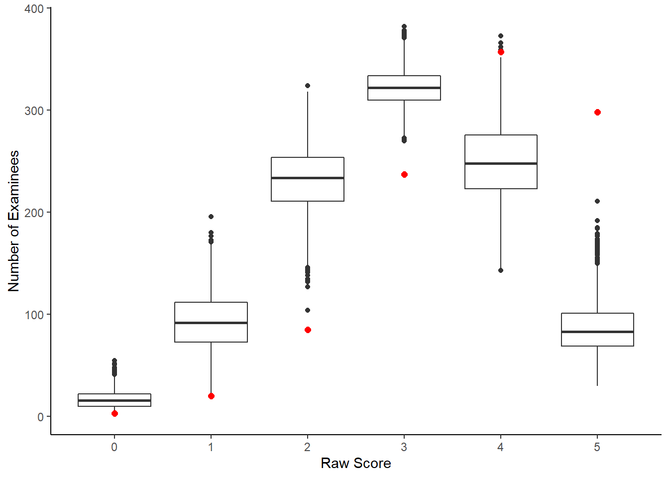

# by item
d <- dat_long %>%
  group_by(chain, iter, person) %>%
  mutate(raw.score = sum(x),
         raw.score.ppd = sum(x.ppd))

di <- d %>%
  filter(chain==1, iter==1001) %>%
  group_by(raw.score, item) %>%
  summarise(p.correct = mean(x))

## `summarise()` has grouped output by 'raw.score'. You can override using the `.groups` argument.

dii <- d %>%
  group_by(chain, iter, raw.score.ppd, item)%>%
  summarise(p.correct = mean(x.ppd))

## `summarise()` has grouped output by 'chain', 'iter', 'raw.score.ppd'. You can override using the
## `.groups` argument.

ggplot()+
  geom_boxplot(data=dii,
               aes(y= p.correct,
                   x= raw.score.ppd,
                   group=raw.score.ppd))+
  geom_point(data=di,
             aes(x=raw.score, y=p.correct),
             color="red", size=2)+
  facet_wrap(.~item)+
  labs(x="Raw Score", y="Number of Examinees")+
  theme_classic()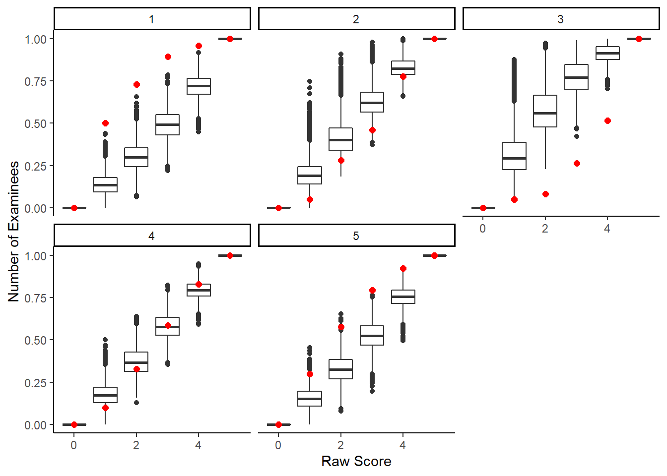

# computing standardized model summary statistics
# objects for results
J <- 5
n.chain <- 3
n.iters <- length(unique(dat_long$iter))
n.iters <- length(unique(long_dat$iter))

## Error in unique(long_dat$iter): object 'long_dat' not found

n.iters.PPMC <- n.iters*n.chain

realized.SMBC.array <- array(NA, c(n.iters.PPMC, J, J))
postpred.SMBC.array <- array(NA, c(n.iters.PPMC, J, J))
realized.SGDDM.vector <- array(NA, c(n.iters.PPMC))
postpred.SGDDM.vector <- array(NA, c(n.iters.PPMC))



ii <- i <- c <- 1
# iteration condiitons
iter.cond <- unique(dat_long$iter)
Xobs <- as.matrix(dat[,-6])

for(i in 1:length(iter.cond)){
  for(c in 1:3){
  cc <- iter.cond[i]
  Xexp <- dat_long[dat_long$chain==c & dat_long$iter==cc , ] %>%
    pivot_wider(
      id_cols = person,
      names_from = "item",
      values_from = "x.exp",
      names_prefix = "item"
    ) %>%
    ungroup()%>%
    select(item1:item5)%>%
    as.matrix()
  Xppd <- dat_long[dat_long$chain==c & dat_long$iter==cc , ] %>%
    pivot_wider(
      id_cols = person,
      names_from = "item",
      values_from = "x.ppd",
      names_prefix = "item"
    ) %>%
    ungroup()%>%
    select(item1:item5)%>%
    as.matrix()

  # compute realized values
  realized.SMBC.array[ii, ,] <- calculate.SMBC.matrix(Xobs, Xexp)
  realized.SGDDM.vector[ii] <-  calculate.SGDDM(Xobs, Xexp)
  # compute PPD values
  postpred.SMBC.array[ii, ,] <- calculate.SMBC.matrix(Xppd, Xexp)
  postpred.SGDDM.vector[ii] <-  calculate.SGDDM(Xppd, Xexp)
    ii <- ii + 1
  }
}


plot.dat.ppd <- data.frame(
  real = realized.SGDDM.vector,
  ppd = postpred.SGDDM.vector
)


ggplot(plot.dat.ppd, aes(x=real, y=ppd))+
  geom_point()+
  geom_abline(intercept = 0, slope=1)+
  lims(x=c(0,0.5), y=c(0, 0.5))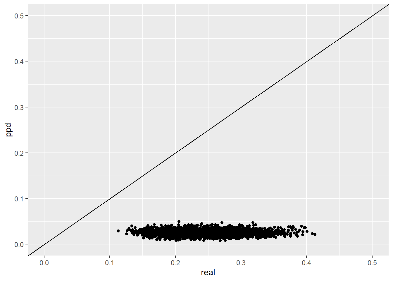

# transform smbc into plotable format
ddim <- dim(postpred.SMBC.array)
plot.dat.ppd <- as.data.frame(matrix(0, nrow=ddim[1]*ddim[2]*ddim[3], ncol=4))
colnames(plot.dat.ppd) <- c("itemj", "itemjj", "real", "ppd")
ii <- i <- j <- jj <- 1

for(i in 1:ddim[1]){
  for(j in 1:ddim[2]){
    for(jj in 1:ddim[3]){
      plot.dat.ppd[ii, 1] <- j
      plot.dat.ppd[ii, 2] <- jj
      plot.dat.ppd[ii, 3] <- realized.SMBC.array[i, j, jj]
      plot.dat.ppd[ii, 4] <- postpred.SMBC.array[i, j, jj]
      ii <- ii + 1
    }
  }
}

plot.dat.ppd <- plot.dat.ppd %>%
  filter(itemj < itemjj) %>%
  mutate(
    cov = paste0("cov(", itemj, ", ", itemjj,")")
  )

ggplot(plot.dat.ppd, aes(x=real, y=ppd))+
  geom_point(alpha=0.25)+
  geom_density2d(adjust=2)+
  geom_abline(intercept = 0, slope=1)+
  facet_wrap(.~cov)+
  lims(x=c(-1,1), y=c(-1,1))+
  theme_classic()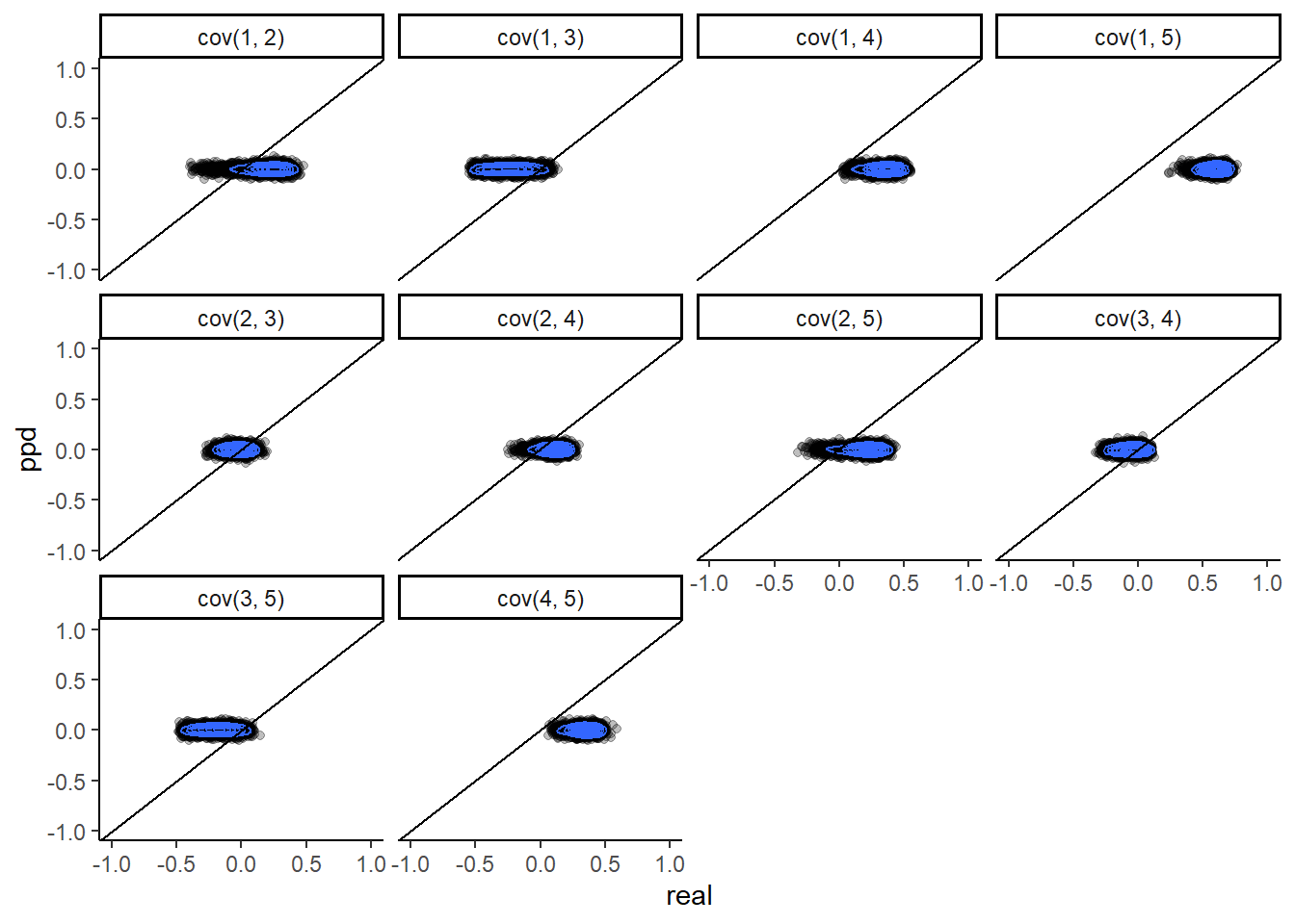

11.4 LSAT Example - Stan

model_irt_lsat <- '
data {
  int  N;
  int  J;
  int x[N,J];
}

parameters {
  real<lower=0> a[J]; //discrimination
  real d[J]; //location
  real<lower=0, upper=1> c[J]; //guessing
  real theta[N]; //person parameters
}

model {
  matrix[N,J] pi;
  // item response probabilities
  for(n in 1:N){
    for(j in 1:J){
      pi[n,j] = c[j]+(1-c[j])*Phi(a[j]*theta[n]+d[j]);
      x[n,j] ~ bernoulli(pi[n,j]);
    }
  }
  //measurement model priors
  for(j in 1:J){
    a[j] ~ normal(1,2)T[0,];
    d[j] ~ normal(0,2);
    c[j] ~ beta(5, 17);
  }
  theta ~ normal(0,1);
}

'


# initial values
start_values <- list(
  list("d"=c(1.00, 1.00, 1.00, 1.00, 1.00),
       "a"=c(1.00, 1.00, 1.00, 1.00, 1.00),
       "c"=c(0.20, 0.20, 0.20, 0.20, 0.20)),
  list("d"=c(-3.00, -3.00, -3.00, -3.00, -3.00),
       "a"=c(3.00, 3.00, 3.00, 3.00, 3.00),
       "c"=c(0.50, 0.50, 0.50, 0.50, 0.50)),
  list("d"=c(3.00, 3.00, 3.00, 3.00, 3.00),
       "a"=c(0.1, 0.1, 0.1, 0.1, 0.1),
       "c"=c(0.05, 0.05, 0.05, 0.05, 0.05))
)

# dataset
dat <- read.table("data/LSAT.dat", header=T)


mydata <- list(
  N = nrow(dat), 
  J = ncol(dat),
  x = as.matrix(dat)
)



# Next, need to fit the model
#   I have explicitly outlined some common parameters
fit <- stan(
  model_code = model_irt_lsat, # model code to be compiled
  data = mydata,          # my data
  init = start_values,    # starting values
  chains = 3,             # number of Markov chains
  warmup = 2000,          # number of warm up iterations per chain
  iter = 4300,            # total number of iterations per chain
  cores = 1,              # number of cores (could use one per chain)
  refresh = 0             # no progress shown
)

## Warning: Bulk Effective Samples Size (ESS) is too low, indicating posterior means and medians may be unreliable.
## Running the chains for more iterations may help. See
## https://mc-stan.org/misc/warnings.html#bulk-ess

# first get a basic breakdown of the posteriors
print(fit,pars =c("d", "a", "c", "theta[1000]"))

## Inference for Stan model: anon_model.
## 3 chains, each with iter=200; warmup=100; thin=1; 
## post-warmup draws per chain=100, total post-warmup draws=300.
## 
##              mean se_mean   sd  2.5%   25%   50%   75% 97.5% n_eff Rhat
## d[1]         1.48    0.04 0.27  1.20  1.35  1.42  1.53  2.00    38 1.05
## d[2]         0.26    0.03 0.29 -0.41  0.18  0.32  0.42  0.55    86 1.02
## d[3]        -0.78    0.13 0.76 -2.80 -1.09 -0.53 -0.25  0.03    32 1.22
## d[4]         0.52    0.01 0.15  0.13  0.45  0.54  0.62  0.73   526 1.00
## d[5]         1.04    0.01 0.12  0.78  0.97  1.04  1.12  1.23   160 1.00
## a[1]         0.55    0.06 0.32  0.24  0.38  0.50  0.63  1.24    27 1.08
## a[2]         0.62    0.05 0.34  0.24  0.43  0.55  0.71  1.48    47 1.04
## a[3]         1.44    0.20 0.99  0.44  0.71  1.08  1.90  3.76    24 1.19
## a[4]         0.48    0.02 0.18  0.17  0.36  0.45  0.59  0.89    61 1.09
## a[5]         0.44    0.02 0.16  0.20  0.33  0.42  0.55  0.80    43 1.09
## c[1]         0.24    0.00 0.09  0.10  0.19  0.23  0.29  0.44   743 0.99
## c[2]         0.26    0.01 0.11  0.09  0.18  0.25  0.33  0.51   197 1.00
## c[3]         0.29    0.01 0.09  0.10  0.22  0.30  0.35  0.45    51 1.12
## c[4]         0.25    0.00 0.10  0.09  0.18  0.25  0.30  0.47   743 1.00
## c[5]         0.24    0.00 0.08  0.10  0.19  0.23  0.29  0.43   743 1.00
## theta[1000]  0.78    0.04 0.93 -1.13  0.20  0.75  1.41  2.48   624 0.99
## 
## Samples were drawn using NUTS(diag_e) at Sun Jul 24 14:56:32 2022.
## For each parameter, n_eff is a crude measure of effective sample size,
## and Rhat is the potential scale reduction factor on split chains (at 
## convergence, Rhat=1).

# plot the posterior in a
#  95% probability interval
#  and 80% to contrast the dispersion
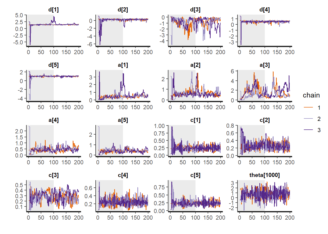
plot(fit,pars =c("d", "a", "c", "theta[1000]"))

## ci_level: 0.8 (80% intervals)

## outer_level: 0.95 (95% intervals)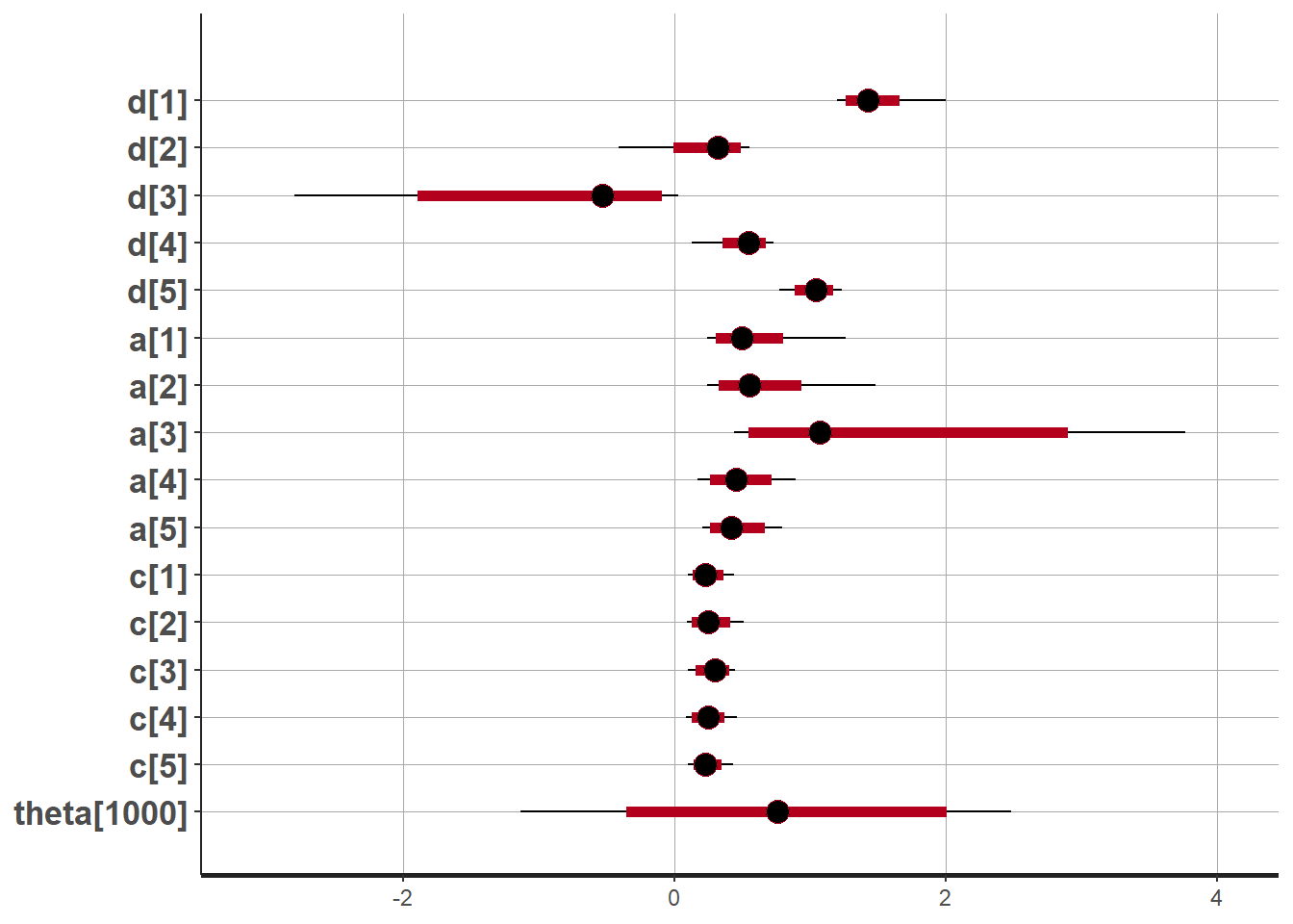

# traceplots
rstan::traceplot(fit,pars =c("d", "a", "c", "theta[1000]"), inc_warmup = TRUE)

# Gelman-Rubin-Brooks Convergence Criterion
ggs_grb(ggs(fit, family = c("d"))) +
   theme_bw() + theme(panel.grid = element_blank())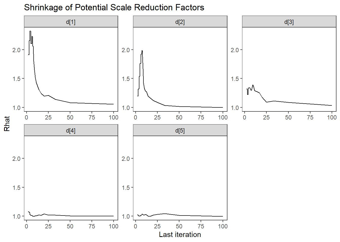

ggs_grb(ggs(fit, family = "a")) +
   theme_bw() + theme(panel.grid = element_blank())

ggs_grb(ggs(fit, family = "c")) +
   theme_bw() + theme(panel.grid = element_blank())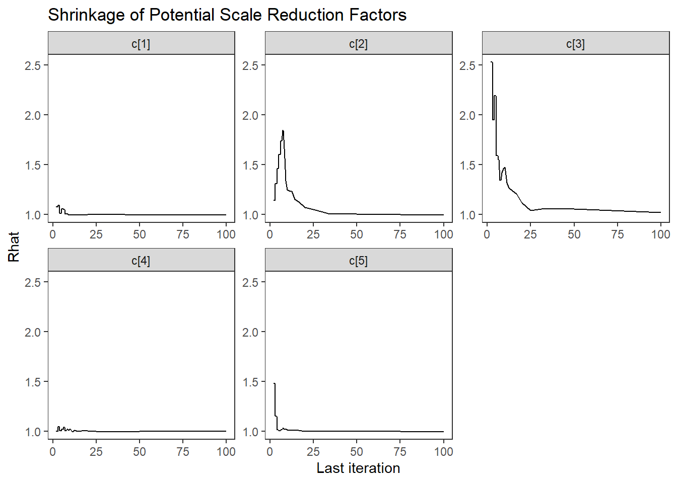

ggs_grb(ggs(fit, family = "theta[1000]")) +
   theme_bw() + theme(panel.grid = element_blank())

## Warning in max(D$Iteration): no non-missing arguments to max; returning -Inf

## Error in ggs_grb(ggs(fit, family = "theta[1000]")): At least two chains are required

# autocorrelation
ggs_autocorrelation(ggs(fit, family="d")) +
   theme_bw() + theme(panel.grid = element_blank())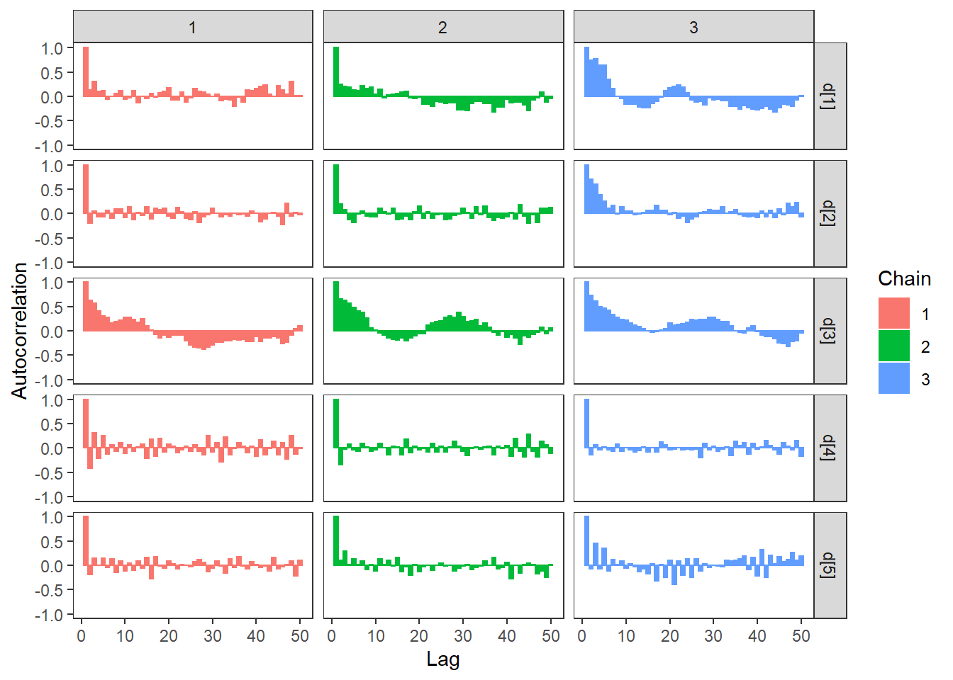

ggs_autocorrelation(ggs(fit, family="a")) +
   theme_bw() + theme(panel.grid = element_blank())

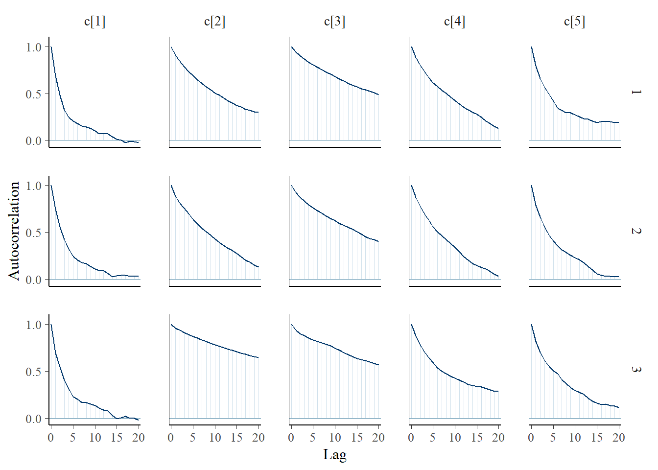
ggs_autocorrelation(ggs(fit, family="c")) +
   theme_bw() + theme(panel.grid = element_blank())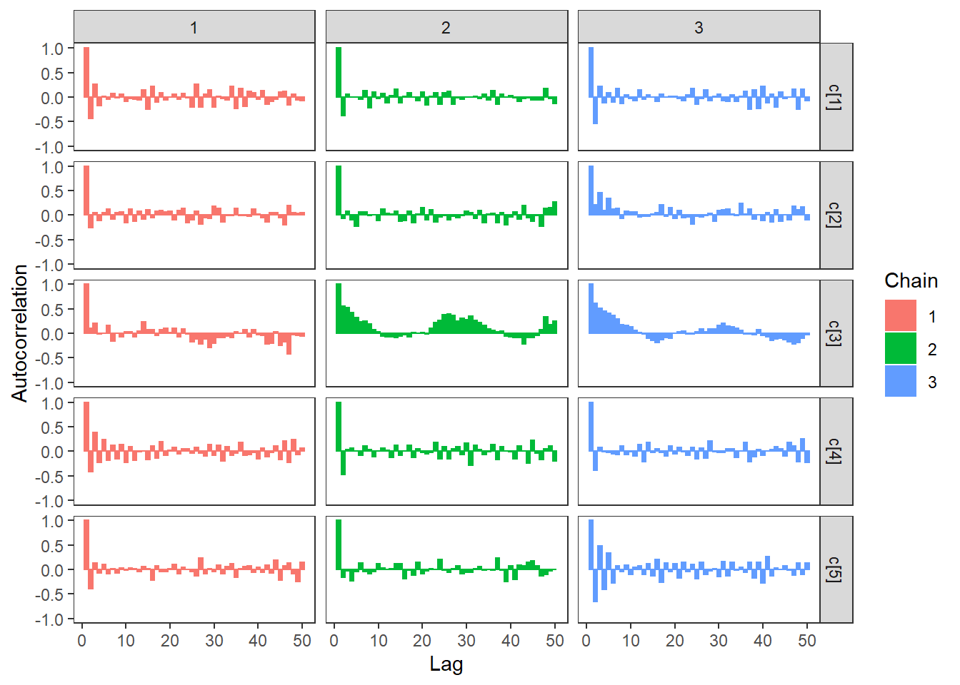

ggs_autocorrelation(ggs(fit, family="theta[1000]")) +
   theme_bw() + theme(panel.grid = element_blank())

## Warning in max(D$Iteration): no non-missing arguments to max; returning -Inf

## Error in sprintf("nLags=%d is larger than number of iterations, computing until max possible lag %d", : invalid format '%d'; use format %f, %e, %g or %a for numeric objects

# plot the posterior density
plot.data <- as.matrix(fit)

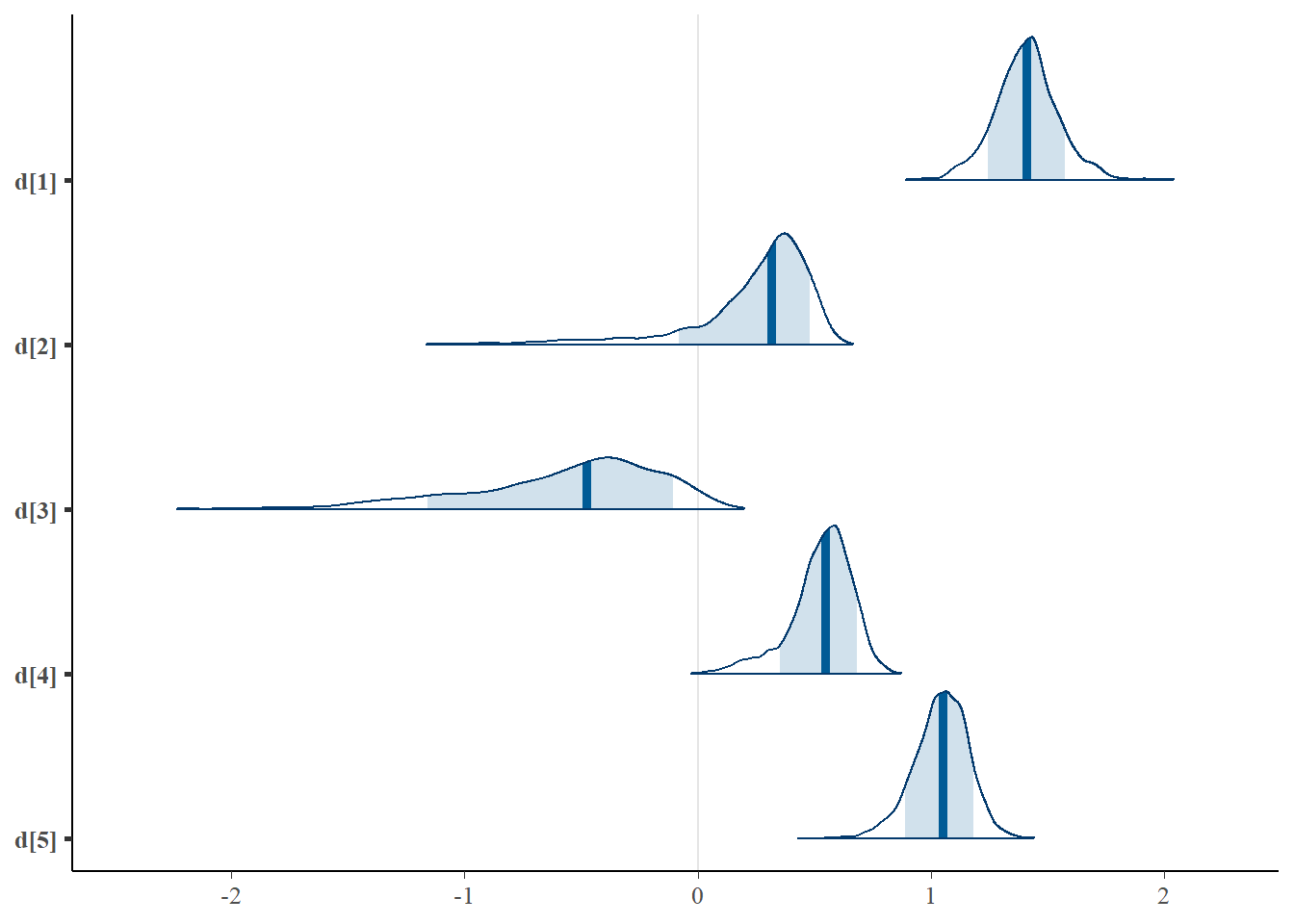
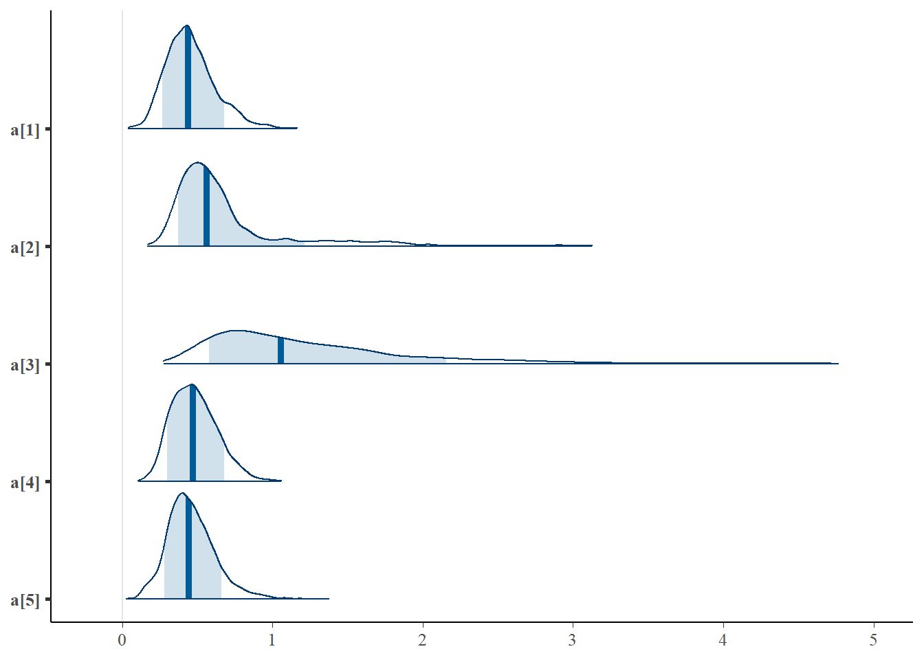
mcmc_areas(plot.data, pars = paste0("d[",1:5,"]"),prob = 0.8)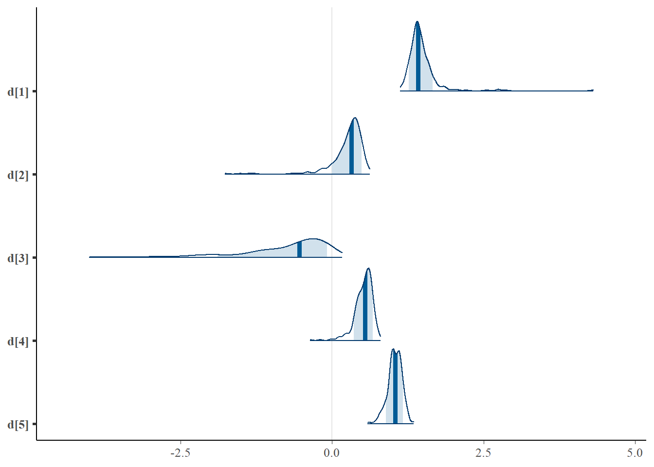

mcmc_areas(plot.data, pars = paste0("a[",1:5,"]"),prob = 0.8)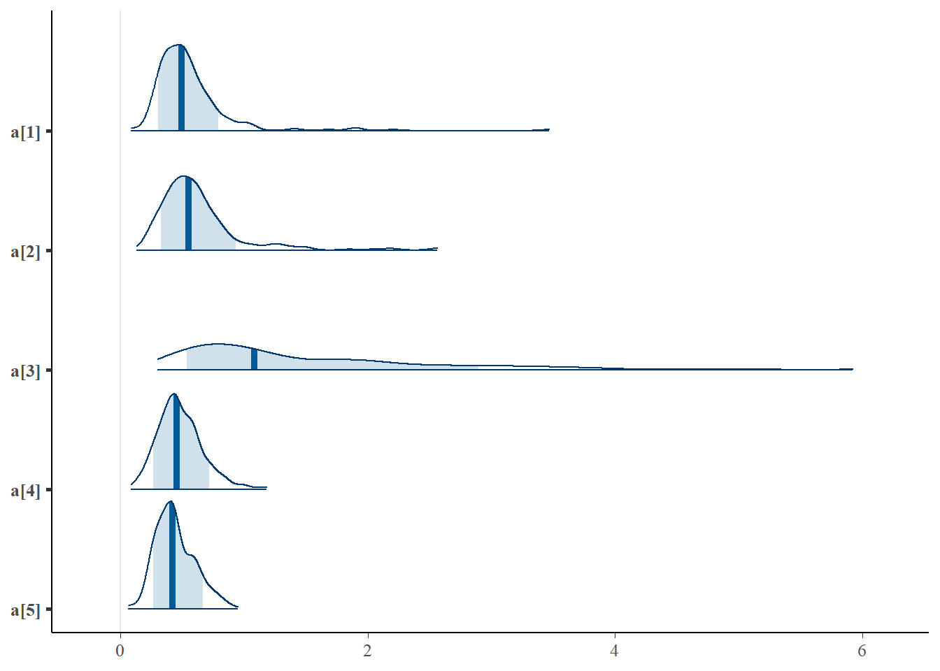

mcmc_areas(plot.data, pars = paste0("c[",1:5,"]"),prob = 0.8)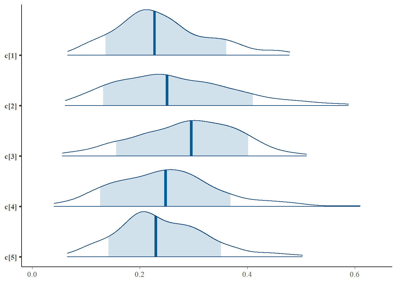

mcmc_areas(plot.data, pars = paste0("theta[1000]"),prob = 0.8)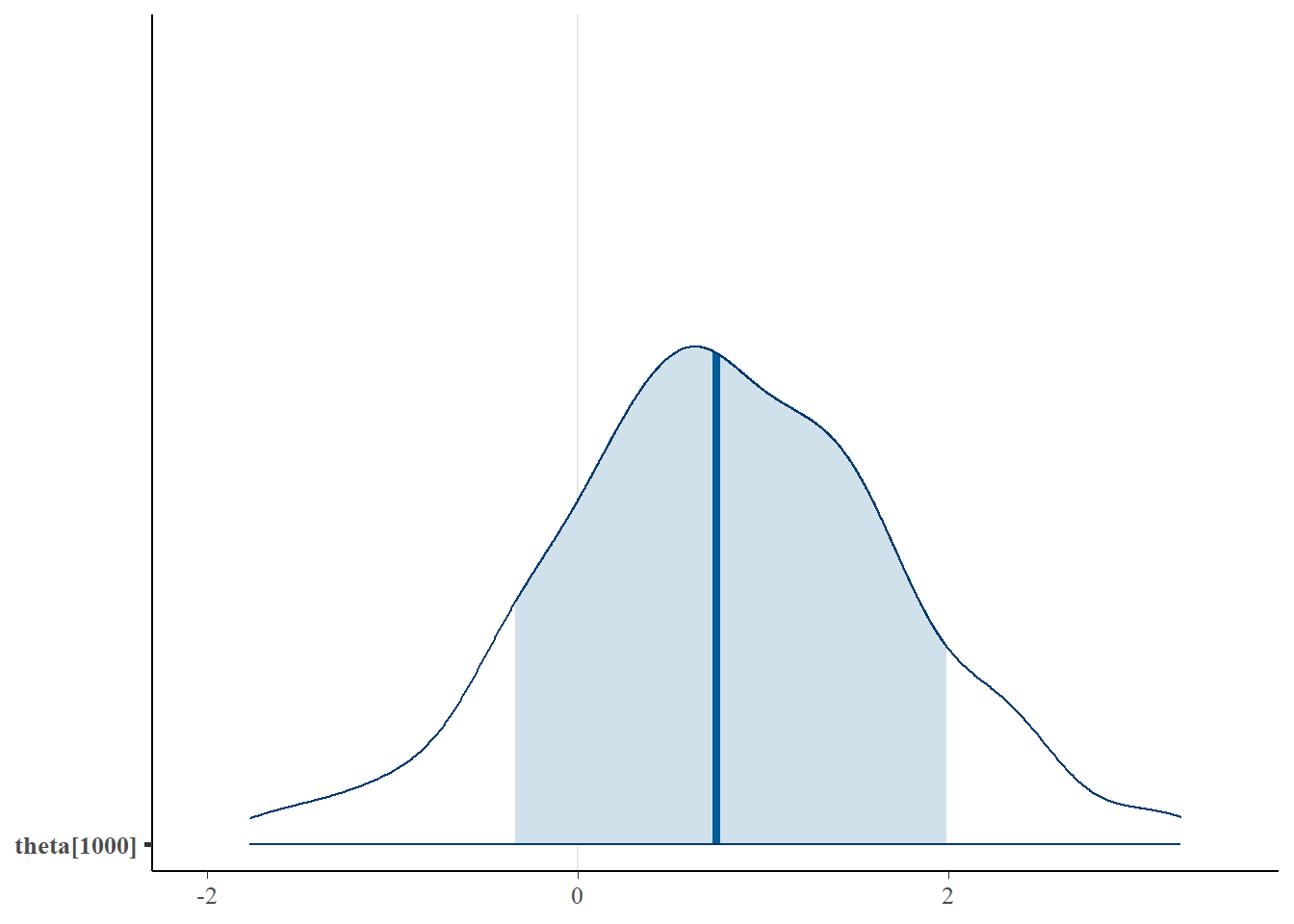

11.5 IRT Models for Polytomous Data

A commonly used IRT model for polytomous items is the graded response model (GRM). Below is one way of describing the model. Let \(x_{ij}\) be the observed response to item \(j\) from examinee \(i\) that may take on values 1, 2, …, \(K_j\), where \(K_j\) is the number of possible responses/outcomes for item \(j\). In many applications, the number of response options is constant across items, though this need not be the case. The GRM using conditional probability statements about the probability of a response being at or above a specific category and obtaining the probability for each category as a difference of two such conditional probabilities. That is \[P(x_{ij} = k \mid \theta_i, \boldsymbol{d}_j,a_j) = P(x_{ij} \geq k \mid \theta_i, d_{jk},a_j) - P(x_{ij} \geq k+1 \mid \theta_i, d_{j(k+1)},a_j),\] where \(\boldsymbol{d}_j\) is the collection of location/threshold parameters for item \(j\). The GRM takes on a structure similar to the 2-PL for any one category \[P(x_{ij} \geq k \mid \theta_i, d_{jk},a_j)=F(a_j\theta_i + d_{jk}).\]

The conditional probability of observed responses may be modeled similarly as we have used for dichotomous responses but with a few important differences. The conditional distribution of the data is \[p(\boldsymbol{x}\mid \boldsymbol{\theta},\boldsymbol{\omega}) = \prod_{i=1}^np(\boldsymbol{x}_i\mid \theta_i, \boldsymbol{\omega}) = \prod_{i=1}^n\prod_{j=1}^Jp(x_{ij}\mid \theta_i, \boldsymbol{\omega}_j),\] where each \(x_{ij}\) is specified as a categorical random variable (or multinomial). A categorical random variable is a generalization of the Bernoulli distribution which is defined be the collection of category response probabilities \[x_{ij} \sim \mathrm{Categorical}(\boldsymbol{P}(x_{ij}\mid\theta_i, \boldsymbol{\omega}_j)).\]

The above helps form the likelihood of the observed data. Next, the prior distribution is described because what the structure should be is not necessarily obvious.

First, the prior for the latent ability follows the same logic from the dichotomous model. We employ an exchangeability assumption to specify independent priors for each respondent with a normally distribution prior.

Next, the measurement model parameters’ priors are described. We again can assume exchangeability and arrive at a common but independent prior across items, and assume that the priors for the location and discrimination parameters are independent. These assumptions may not be tenable in theory, but they are practically useful. The priors for discrimination stay the same as the dichotomous model. The priors for the location parameters are a bit more involved.

For the location parameters, the first location parameter \(d_{j1}\) specifies the probability of responding a 1 or greater which is a certainty if they gave a response. Therefore, the probability would be 1. We set \(d_{j1} = -\inf\) and then set a normal prior for \(d_{j2}\sim \mathrm{Normal}(\mu_{d2},\sigma^2_{d2})\). The priors for the remaining location parameters (\(d_{3}-d_{k}\)) can be specified as truncated normal distributions. That is, the location of the next threshold is constrained to be larger than the previous threshold and is formally \[d_{jk} \sim \mathrm{Normal}^{>d_{j(k-1)}}(\mu_{d_k},\sigma^2_{d_k}),\ \mathrm{for}\ k=3, ...,K_j.\]

The posterior distribution for the GRM can be parameterized as follows. The model as described below is very general and can accommodate varying number of thresholds per item but is constrained to only 1 latent factor.

\[p(\boldsymbol{\theta}, \boldsymbol{d}, \boldsymbol{a}\mid \mathbf{x}) \propto \prod_{i=1}^n\prod_{j=1}^Jp(\theta_i\mid\theta_i, \boldsymbol{d}_j, a_j)p(\theta_i)p(a_j)\prod_{k=2}^{K_j}p(d_{jk}),\] where \[\begin{align*} x_{ij}\mid\theta_i\mid\theta_i, \boldsymbol{d}_j, a_j) &\sim \mathrm{Categorical}(\boldsymbol{P}(x_{ij}\mid\theta_i, \boldsymbol{\omega}_j)),\ \mathrm{for}\ i=1, \cdots, n,\ j = 1, \cdots, J;\\ \mathbf{P}(x_{ij}\mid\theta_i, \boldsymbol{d}_j, a_j) &= \left(P(x_{ij}=1\mid\theta_i, \boldsymbol{d}_j, a_j), \cdots, P(x_{ij}=K_j\mid\theta_i, \boldsymbol{d}_j, a_j)\right),\ \mathrm{for}\ i=1, \cdots, n,\ j = 1, \cdots, J;\\ P(x_{ij}=k\mid\theta_i, \boldsymbol{d}_j, a_j) &= P(x_{ij}\geq k\mid\theta_i,d_{jk}, a_j) - P(x_{ij}\geq k+1\mid\theta_i, d_{j(k+1)}, a_j),\ \mathrm{for}\ i=1, \cdots, n,\ j = 1, \cdots, J,\ k = 1,\cdots,K_j-1;\\ P(x_{ij}=K_j\mid\theta_i, \boldsymbol{d}_j, a_j) &= P(x_{ij}\geq K_j\mid\theta_i,d_{jK_j}, a_j),\ \mathrm{for}\ i=1, \cdots, n,\ j = 1, \cdots, J;\\ P(x_{ij}\geq k\mid\theta_i, d_{jk}, a_j) &= F(a_j\theta_j + d_{jk}),\ \mathrm{for}\ i=1, \cdots, n,\ j = 1, \cdots, J,\ k=2,\cdots,K_j;\\ P(x_{ij}\geq 1\mid\theta_i, d_{j1}, a_j) &= 1,\ \mathrm{for}\ i=1, \cdots, n,\ j = 1, \cdots, J;\\ \theta_i \mid \mu_{\theta}, \sigma^2_{\theta} &\sim \mathrm{Normal}(\mu_{\theta}, \sigma^2_{\theta}),\ \mathrm{for}\ i = 1, \cdots, n;\\ a_j \mid \mu_{a}, \sigma^2_{a} &\sim \mathrm{Normal}^{+}(\mu_{a}, \sigma^2_{a}),\ \mathrm{for}\ j=1, \cdots, J;\\ d_{j2}\mid\mu_{j2}, \sigma^2_{j2} &\sim \mathrm{Normal}(\mu_{j2}, \sigma^2_{j2} ),\ \mathrm{for}\ j=1, \cdots, J;\ \mathrm{and}\\ d_{jk}\mid\mu_{d_{jk}},\sigma^2_{d_{jk}} &\sim \mathrm{Normal}^{>d_{j(k-1)}}(\mu_{d_{jk}},\sigma^2_{d_{jk}}),\ \mathrm{for}\ j=1, \cdots, J,\ k=3, ...,K_j. \end{align*}\]

11.6 GRM Peer Interactions Example

The book uses an example of Peer Interactions from 500 responses to seven items. All the responses are coded from 1 to 5 on an agreement Likert-type scale. A DAG for the GRM corresponding to these data is shown below.

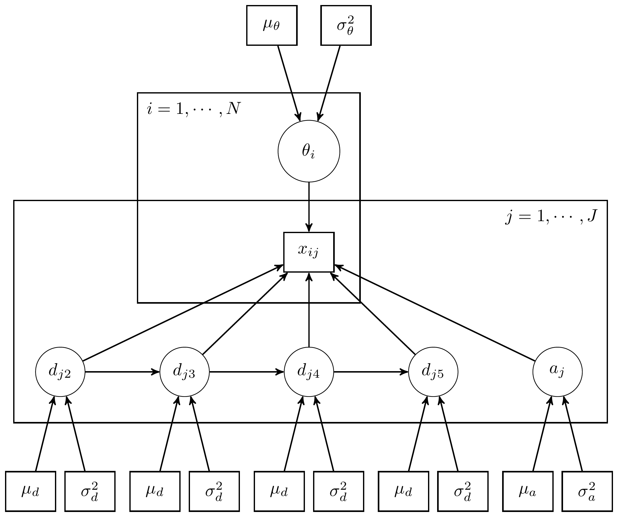
Figure 11.4: DAG for the for Peer Interactions GRM analysis

The path diagram version is substantially simpler and identical to the path diagram for the 3-PL and factor analysis diagrams. Highlighting the similarity in substantive modeling of polytomous items to dichotomous items.

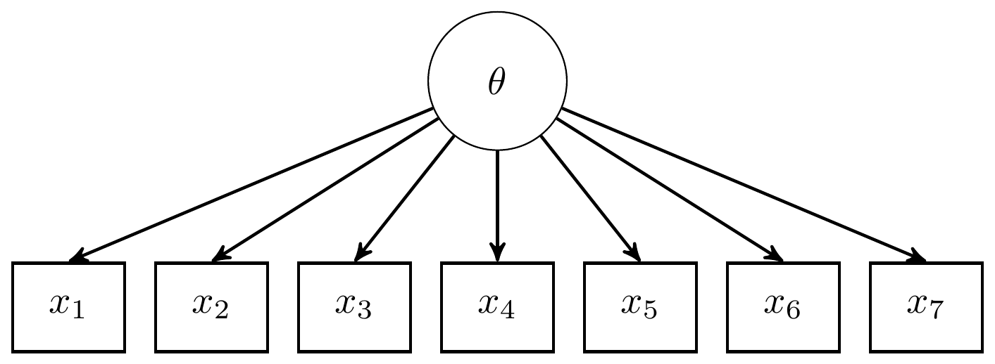
Figure 11.5: Path diagram for the Peer Interactions GRM analysis

For completeness, I have included the model specification diagram that more concretely connects the DAG and path diagram to the assumed distributions and priors.

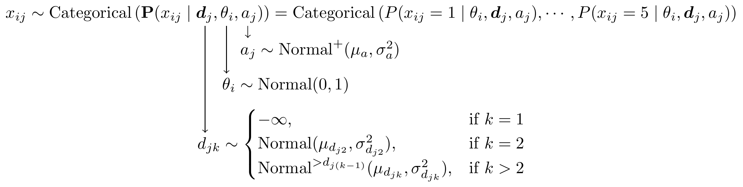
Figure 11.6: Model specification diagram for the Peer Interactions GRM analysis

11.6.1 Example Specific Model Specification

In fitting the GRM to the Peer Interactions data, we can be more precise about the prior and likelihood structure. Below is a breakdown of the model specific to this example. Everything is structurally identical to the previous page but specific values are chosen for the hyperparameters.

\[p(\boldsymbol{\theta}, \boldsymbol{d}, \boldsymbol{a}\mid \mathbf{x}) \propto \prod_{i=1}^n\prod_{j=1}^Jp(\theta_i\mid\theta_i, \boldsymbol{d}_j, a_j)p(\theta_i)p(a_j)\prod_{k=2}^{K_j}p(d_{jk}),\] where \[\begin{align*} x_{ij}\mid\theta_i\mid\theta_i, \boldsymbol{d}_j, a_j) &\sim \mathrm{Categorical}(\boldsymbol{P}(x_{ij}\mid\theta_i, \boldsymbol{\omega}_j)),\ \mathrm{for}\ i=1, \cdots, 500,\ j = 1, \cdots, 7;\\ \mathbf{P}(x_{ij}\mid\theta_i, \boldsymbol{d}_j, a_j) &= \left(P(x_{ij}=1\mid\theta_i, \boldsymbol{d}_j, a_j), \cdots, P(x_{ij}=5\mid\theta_i, \boldsymbol{d}_j, a_j)\right),\ \mathrm{for}\ i=1, \cdots, 500,\ j = 1, \cdots, 7;\\ P(x_{ij}=k\mid\theta_i, \boldsymbol{d}_j, a_j) &= P(x_{ij}\geq k\mid\theta_i,d_{jk}, a_j) - P(x_{ij}\geq k+1\mid\theta_i, d_{j(k+1)}, a_j),\ \mathrm{for}\ i=1, \cdots, 500,\ j = 1, \cdots, 7,\ k = 1,\cdots,4;\\ P(x_{ij}=5\mid\theta_i, \boldsymbol{d}_j, a_j) &= P(x_{ij}\geq 5\mid\theta_i,d_{j5}, a_j),\ \mathrm{for}\ i=1, \cdots, 500,\ j = 1, \cdots, 7;\\ P(x_{ij}\geq k\mid\theta_i, d_{jk}, a_j) &= F(a_j\theta_j + d_{jk}) = \frac{\exp\left(a_j\theta_i +d_{jk}\right)}{1+\exp\left(a_j\theta_i +d_{jk}\right)},\ \mathrm{for}\ i=1, \cdots, 500,\ j = 1, \cdots, 7,\ k=2,\cdots,5;\\ P(x_{ij}\geq 1\mid\theta_i, d_{j1}, a_j) &= 1,\ \mathrm{for}\ i=1, \cdots, 500,\ j = 1, \cdots, 7;\\ \theta_i \mid \mu_{\theta}, \sigma^2_{\theta} &\sim \mathrm{Normal}(0, 1),\ \mathrm{for}\ i = 1, \cdots, 500;\\ a_j \mid \mu_{a}, \sigma^2_{a} &\sim \mathrm{Normal}^{+}(0,2),\ \mathrm{for}\ j=1, \cdots, 7;\\ d_{j2}\mid\mu_{d_{j2}}, \sigma^2_{d_{j2}} &\sim \mathrm{Normal}(2,2),\ \mathrm{for}\ j=1, \cdots, 7;\\ d_{j3}\mid\mu_{d_{j3}},\sigma^2_{d_{j3}} &\sim \mathrm{Normal}^{>d_{j2}}(1, 2),\ \mathrm{for}\ j=1, \cdots, 7;\\ d_{j4}\mid\mu_{d_{j4}},\sigma^2_{d_{j4}} &\sim \mathrm{Normal}^{>d_{j3}}(-1, 2),\ \mathrm{for}\ j=1, \cdots, 7; \mathrm{and}\\ d_{j5}\mid\mu_{d_{j5}},\sigma^2_{d_{j5}} &\sim \mathrm{Normal}^{>d_{j4}}(-2, 2),\ \mathrm{for}\ j=1, \cdots, 7. \end{align*}\]

11.7 PI Example - JAGS

In the below implementation, I had to change d[j,3] ~ dnorm(1, .5)I(d[j,4],d[j,2]) to d[j,3] ~ dnorm(1, .5);I(,d[j,2]) because (1) R is dumb and doesn’t realize that I is a JAGS function; and (2) JAGS does not allow for a directed cycle. The directed cycle in the DAG is when the range of values for d[j,3] is fixed to be within I(d[j,4],d[j,2]) and is not permissible. We need to simply constrain the thresholds to be decreasing or smaller than the previous threshold. I’m not sure of the underlying technical reason for this error, but I found that adding the semi-colon fixes the issue when defining the model as an R function.

jags.model.peer.int <- function(){

  #######################################
  # Specify the item response measurement model for the observables
  #######################################
  for (i in 1:n){
    for(j in 1:J){
  
      ###################################
      # Specify the probabilities of a value being greater than or equal to each category
      ###################################
      for(k in 2:(K[j])){
        # P(greater than or equal to category k > 1)
        logit(P.gte[i,j,k]) <- a[j]*theta[i]+d[j,k]
      }
      # P(greater than or equal to category 1)
      P.gte[i,j,1] <- 1
  
  
      ###################################
      # Specify the probabilities of a value being equal to each category
      ###################################
      for(k in 1:(K[j]-1)){
        # P(greater equal to category k < K)
        P[i,j,k] <- P.gte[i,j,k]-P.gte[i,j,k+1]
      }
      # P(greater equal to category K)
      P[i,j,K[j]] <- P.gte[i,j,K[j]]
      
      ###################################
      # Specify the distribution for each observable
      ###################################
      x[i,j] ~ dcat(P[i,j,1:K[j]])
    }
  }
  
  
  #######################################
  # Specify the (prior) distribution for the latent variables
  #######################################
  for (i in 1:n){
    theta[i] ~ dnorm(0, 1)  # distribution for the latent variables
  }
  
  
  #######################################
  # Specify the prior distribution for the measurement model parameters
  #######################################
  for(j in 1:J){
    
    d[j,2] ~ dnorm(2, .5)                   # Locations for k = 2
    d[j,3] ~ dnorm(1, .5);I(,d[j,2])   # Locations for k = 3
    d[j,4] ~ dnorm(-1, .5);I(,d[j,3])  # Locations for k = 4
    d[j,5] ~ dnorm(-2, .5);I(,d[j,4])        # Locations for k = 5
    a[j] ~ dnorm(1, .5); I(0,)    # Discriminations for observables
  
  }

} # closes the model

# initial values
start_values <- list(
  list(
    d= matrix(c(NA, 3.00E+00, 1.00E+00, 0.00E+00, -1.00E+00,
               NA, 3.00E+00, 1.00E+00, 0.00E+00, -1.00E+00,
               NA, 3.00E+00, 1.00E+00, 0.00E+00, -1.00E+00,
               NA, 3.00E+00, 1.00E+00, 0.00E+00, -1.00E+00,
               NA, 3.00E+00, 1.00E+00, 0.00E+00, -1.00E+00,
               NA, 3.00E+00, 1.00E+00, 0.00E+00, -1.00E+00,
               NA, 3.00E+00, 1.00E+00, 0.00E+00, -1.00E+00),
      ncol=5, nrow=7, byrow=T),
    a=c(1.00E-01, 1.00E-01, 1.00E-01, 1.00E-01, 1.00E-01, 1.00E-01, 1.00E-01)),
  list(
    d= matrix(c(NA, 2.00E+00, 0.00E+00, -1.00E+00, -2.00E+00,
               NA, 2.00E+00, 0.00E+00, -1.00E+00, -2.00E+00,
               NA, 2.00E+00, 0.00E+00, -1.00E+00, -2.00E+00,
               NA, 2.00E+00, 0.00E+00, -1.00E+00, -2.00E+00,
               NA, 2.00E+00, 0.00E+00, -1.00E+00, -2.00E+00,
               NA, 2.00E+00, 0.00E+00, -1.00E+00, -2.00E+00,
               NA, 2.00E+00, 0.00E+00, -1.00E+00, -2.00E+00),
      ncol=5, nrow=7, byrow=T),
    a=c(3.00E+00, 3.00E+00, 3.00E+00, 3.00E+00, 3.00E+00, 3.00E+00, 3.00E+00)),
  list(
    d= matrix(c(NA, 1.00E+00, -1.00E+00, -2.00E+00, -3.00E+00,
               NA, 1.00E+00, -1.00E+00, -2.00E+00, -3.00E+00,
               NA, 1.00E+00, -1.00E+00, -2.00E+00, -3.00E+00,
               NA, 1.00E+00, -1.00E+00, -2.00E+00, -3.00E+00,
               NA, 1.00E+00, -1.00E+00, -2.00E+00, -3.00E+00,
               NA, 1.00E+00, -1.00E+00, -2.00E+00, -3.00E+00,
               NA, 1.00E+00, -1.00E+00, -2.00E+00, -3.00E+00),
              ncol=5, nrow=7, byrow=T),
    a=c(1.00E+00, 1.00E+00, 1.00E+00, 1.00E+00, 1.00E+00, 1.00E+00, 1.00E+00))
)

# vector of all parameters to save
param_save <- c("a", "d", "theta")

# dataset
dat <- read.table("data/PI.dat", header=T)

mydata <- list(
  n = nrow(dat), J = ncol(dat),
  K = rep(5, ncol(dat)),
  x = as.matrix(dat)
)

# fit model
fit <- jags(
  model.file=jags.model.peer.int,
  data=mydata,
  inits=start_values,
  parameters.to.save = param_save,
  n.iter=4000,
  n.burnin = 2000,
  n.chains = 3,
  progress.bar = "none")

## module glm loaded

## Compiling model graph
##    Resolving undeclared variables
##    Allocating nodes
## Graph information:
##    Observed stochastic nodes: 3500
##    Unobserved stochastic nodes: 535
##    Total graph size: 53050
## 
## Initializing model

print(fit)

## Inference for Bugs model at "C:/Users/noahp/AppData/Local/Temp/RtmpoRjxzc/model6f744e4175e6.txt", fit using jags,
##  3 chains, each with 4000 iterations (first 2000 discarded), n.thin = 2
##  n.sims = 3000 iterations saved
##             mu.vect sd.vect     2.5%      25%      50%      75%    97.5%  Rhat n.eff
## a[1]          2.144   0.165    1.834    2.032    2.140    2.254    2.474 1.001  3000
## a[2]          3.522   0.271    2.996    3.336    3.517    3.709    4.049 1.004   730
## a[3]          3.965   0.304    3.403    3.763    3.951    4.156    4.604 1.007   360
## a[4]          3.557   0.258    3.071    3.384    3.548    3.726    4.106 1.024    95
## a[5]          2.461   0.187    2.106    2.336    2.460    2.583    2.832 1.001  2300
## a[6]          1.873   0.147    1.598    1.773    1.865    1.971    2.178 1.001  3000
## a[7]          1.495   0.128    1.246    1.410    1.489    1.580    1.754 1.002  1400
## d[1,2]        4.969   0.332    4.359    4.737    4.959    5.180    5.648 1.003   680
## d[2,2]        5.224   0.384    4.472    4.960    5.225    5.481    5.974 1.004   740
## d[3,2]        6.559   0.471    5.630    6.247    6.549    6.865    7.506 1.003  3000
## d[4,2]        6.386   0.448    5.572    6.063    6.370    6.672    7.304 1.016   140
## d[5,2]        4.817   0.330    4.203    4.584    4.808    5.035    5.498 1.002  1000
## d[6,2]        3.853   0.251    3.389    3.675    3.851    4.013    4.380 1.001  2300
## d[7,2]        4.289   0.295    3.739    4.087    4.272    4.478    4.891 1.006   360
## d[1,3]        2.978   0.207    2.581    2.838    2.975    3.116    3.399 1.003   750
## d[2,3]        1.218   0.209    0.802    1.085    1.220    1.359    1.623 1.011   290
## d[3,3]        3.378   0.305    2.790    3.175    3.373    3.583    3.992 1.002  3000
## d[4,3]        2.731   0.245    2.262    2.565    2.727    2.889    3.231 1.010   210
## d[5,3]        2.720   0.209    2.310    2.578    2.717    2.858    3.137 1.008   310
## d[6,3]        1.979   0.165    1.660    1.872    1.976    2.086    2.306 1.005   530
## d[7,3]        2.462   0.167    2.148    2.347    2.462    2.577    2.801 1.009   250
## d[1,4]        0.676   0.140    0.412    0.578    0.675    0.770    0.952 1.005   440
## d[2,4]       -1.729   0.215   -2.166   -1.865   -1.726   -1.586   -1.323 1.012   180
## d[3,4]       -1.261   0.225   -1.730   -1.403   -1.256   -1.113   -0.831 1.017   160
## d[4,4]       -0.753   0.198   -1.150   -0.884   -0.750   -0.618   -0.381 1.009   310
## d[5,4]       -0.320   0.157   -0.631   -0.422   -0.320   -0.216   -0.006 1.007   330
## d[6,4]       -0.468   0.133   -0.726   -0.559   -0.467   -0.377   -0.211 1.007   320
## d[7,4]        0.285   0.119    0.041    0.208    0.288    0.364    0.508 1.007   330
## d[1,5]       -2.483   0.187   -2.863   -2.610   -2.479   -2.355   -2.134 1.005   510
## d[2,5]       -5.089   0.362   -5.808   -5.338   -5.077   -4.831   -4.420 1.005   420
## d[3,5]       -5.521   0.408   -6.390   -5.778   -5.502   -5.248   -4.751 1.012   210
## d[4,5]       -4.779   0.359   -5.541   -5.006   -4.766   -4.539   -4.123 1.015   150
## d[5,5]       -3.583   0.252   -4.107   -3.745   -3.577   -3.419   -3.104 1.001  2000
## d[6,5]       -3.193   0.209   -3.612   -3.332   -3.189   -3.043   -2.806 1.002  1600
## d[7,5]       -2.723   0.188   -3.090   -2.853   -2.722   -2.587   -2.372 1.002  1300
## theta[1]      0.843   0.277    0.299    0.653    0.847    1.030    1.379 1.002  1300
## theta[2]     -0.987   0.256   -1.493   -1.159   -0.986   -0.818   -0.487 1.001  2200
## theta[3]     -1.047   0.250   -1.551   -1.207   -1.044   -0.880   -0.569 1.001  3000
## theta[4]     -0.264   0.256   -0.761   -0.435   -0.267   -0.090    0.229 1.002  1200
## theta[5]      0.093   0.270   -0.439   -0.090    0.092    0.266    0.640 1.002  1000
## theta[6]      0.093   0.257   -0.422   -0.081    0.098    0.264    0.588 1.003   740
## theta[7]      1.437   0.321    0.827    1.221    1.433    1.641    2.087 1.001  3000
## theta[8]      0.769   0.264    0.260    0.591    0.761    0.950    1.314 1.001  3000
## theta[9]     -0.018   0.252   -0.497   -0.190   -0.021    0.151    0.474 1.002  1400
## theta[10]     0.343   0.271   -0.184    0.168    0.334    0.519    0.891 1.001  3000
## theta[11]    -0.778   0.256   -1.282   -0.944   -0.775   -0.608   -0.275 1.003   720
## theta[12]    -0.205   0.259   -0.722   -0.380   -0.201   -0.028    0.297 1.001  2300
## theta[13]     1.034   0.278    0.492    0.840    1.031    1.225    1.572 1.001  3000
## theta[14]    -0.013   0.255   -0.517   -0.182   -0.012    0.156    0.477 1.001  3000
## theta[15]    -0.711   0.259   -1.224   -0.885   -0.708   -0.545   -0.186 1.002  1300
## theta[16]    -0.452   0.286   -1.009   -0.648   -0.461   -0.266    0.121 1.001  3000
## theta[17]     2.351   0.468    1.574    2.016    2.300    2.635    3.410 1.001  2800
## theta[18]     0.225   0.259   -0.284    0.049    0.227    0.399    0.717 1.003   790
## theta[19]     0.026   0.257   -0.480   -0.146    0.023    0.197    0.534 1.002  1000
## theta[20]     0.227   0.268   -0.299    0.052    0.231    0.404    0.746 1.002  1100
## theta[21]     0.358   0.259   -0.158    0.193    0.358    0.525    0.871 1.002  2100
## theta[22]    -1.029   0.260   -1.548   -1.203   -1.035   -0.859   -0.511 1.004   560
## theta[23]     0.669   0.265    0.157    0.496    0.660    0.835    1.198 1.001  3000
## theta[24]     0.061   0.265   -0.470   -0.121    0.062    0.243    0.553 1.001  3000
## theta[25]     2.349   0.459    1.585    2.021    2.303    2.634    3.383 1.001  3000
## theta[26]     0.538   0.296   -0.038    0.342    0.533    0.730    1.133 1.001  3000
## theta[27]    -0.772   0.265   -1.301   -0.949   -0.775   -0.589   -0.255 1.005   500
## theta[28]     0.194   0.254   -0.305    0.021    0.196    0.365    0.699 1.003   720
## theta[29]     1.054   0.288    0.500    0.859    1.055    1.248    1.633 1.003  2500
## theta[30]     0.357   0.250   -0.133    0.186    0.355    0.522    0.849 1.003   860
## theta[31]     0.476   0.259   -0.022    0.301    0.478    0.645    0.991 1.002  3000
## theta[32]     0.428   0.267   -0.095    0.252    0.432    0.600    0.960 1.001  2800
## theta[33]     0.412   0.267   -0.114    0.238    0.405    0.593    0.919 1.002  1000
## theta[34]     0.126   0.261   -0.390   -0.044    0.127    0.301    0.614 1.002  1800
## theta[35]    -1.319   0.266   -1.839   -1.498   -1.321   -1.138   -0.792 1.001  3000
## theta[36]     0.766   0.267    0.252    0.587    0.767    0.949    1.305 1.001  3000
## theta[37]    -0.533   0.263   -1.047   -0.706   -0.532   -0.356   -0.024 1.001  3000
## theta[38]    -0.737   0.253   -1.227   -0.906   -0.740   -0.568   -0.229 1.001  2700
## theta[39]    -0.468   0.298   -1.047   -0.666   -0.470   -0.266    0.121 1.001  3000
## theta[40]    -0.153   0.265   -0.685   -0.331   -0.146    0.030    0.351 1.002  1900
## theta[41]     0.212   0.277   -0.321    0.026    0.210    0.392    0.770 1.001  3000
## theta[42]    -2.220   0.347   -2.952   -2.442   -2.197   -1.974   -1.594 1.001  3000
## theta[43]     2.082   0.394    1.406    1.804    2.046    2.336    2.934 1.001  3000
## theta[44]    -0.398   0.297   -0.972   -0.599   -0.405   -0.196    0.190 1.001  3000
## theta[45]     2.360   0.469    1.566    2.019    2.315    2.660    3.424 1.001  3000
## theta[46]     0.760   0.259    0.260    0.589    0.760    0.932    1.256 1.001  3000
## theta[47]    -0.858   0.265   -1.374   -1.037   -0.862   -0.684   -0.312 1.001  3000
## theta[48]    -0.197   0.268   -0.721   -0.385   -0.190   -0.016    0.306 1.001  3000
## theta[49]     0.164   0.270   -0.365   -0.009    0.166    0.339    0.690 1.002  1800
## theta[50]    -0.588   0.292   -1.147   -0.782   -0.592   -0.397   -0.001 1.001  3000
## theta[51]    -0.383   0.262   -0.886   -0.567   -0.376   -0.209    0.128 1.002  1600
## theta[52]    -1.026   0.252   -1.528   -1.197   -1.018   -0.858   -0.540 1.002  1200
## theta[53]     0.434   0.261   -0.078    0.262    0.435    0.604    0.985 1.001  3000
## theta[54]     0.372   0.284   -0.193    0.185    0.376    0.559    0.925 1.002  1800
## theta[55]    -0.850   0.268   -1.386   -1.030   -0.847   -0.673   -0.321 1.001  3000
## theta[56]     0.772   0.255    0.268    0.604    0.774    0.944    1.276 1.002  1800
## theta[57]     1.389   0.275    0.850    1.211    1.383    1.572    1.935 1.003   900
## theta[58]    -0.840   0.259   -1.356   -1.015   -0.837   -0.670   -0.313 1.001  3000
## theta[59]     0.094   0.260   -0.413   -0.084    0.092    0.270    0.619 1.002  1000
## theta[60]     0.337   0.258   -0.178    0.167    0.339    0.495    0.852 1.002  1700
## theta[61]    -1.791   0.297   -2.422   -1.979   -1.786   -1.592   -1.229 1.003   890
## theta[62]    -0.426   0.255   -0.938   -0.594   -0.427   -0.257    0.084 1.001  3000
## theta[63]     2.336   0.469    1.557    2.010    2.282    2.619    3.427 1.001  3000
## theta[64]    -0.935   0.247   -1.423   -1.107   -0.936   -0.766   -0.463 1.002  1200
## theta[65]     0.365   0.265   -0.162    0.191    0.368    0.539    0.872 1.002  1900
## theta[66]     0.774   0.259    0.271    0.599    0.774    0.951    1.279 1.002  2800
## theta[67]     0.337   0.256   -0.148    0.156    0.330    0.506    0.852 1.001  3000
## theta[68]     1.598   0.297    1.045    1.398    1.588    1.789    2.214 1.001  3000
## theta[69]     1.078   0.272    0.552    0.900    1.082    1.255    1.620 1.003   960
## theta[70]     1.614   0.301    1.060    1.406    1.597    1.805    2.249 1.001  2400
## theta[71]    -0.013   0.256   -0.502   -0.189   -0.008    0.162    0.496 1.001  3000
## theta[72]    -1.028   0.258   -1.542   -1.202   -1.021   -0.857   -0.524 1.004   700
## theta[73]     0.140   0.266   -0.378   -0.037    0.139    0.315    0.675 1.001  2100
## theta[74]    -2.309   0.393   -3.175   -2.544   -2.279   -2.030   -1.638 1.002  1000
## theta[75]    -0.135   0.282   -0.693   -0.330   -0.129    0.055    0.415 1.001  3000
## theta[76]    -1.111   0.253   -1.599   -1.279   -1.119   -0.933   -0.612 1.001  2200
##  [ reached getOption("max.print") -- omitted 425 rows ]
## 
## For each parameter, n.eff is a crude measure of effective sample size,
## and Rhat is the potential scale reduction factor (at convergence, Rhat=1).
## 
## DIC info (using the rule, pD = var(deviance)/2)
## pD = 706.9 and DIC = 7026.0
## DIC is an estimate of expected predictive error (lower deviance is better).

round(fit$BUGSoutput$summary[ !rownames(fit$BUGSoutput$summary) %like% "theta", ], 3)

##              mean     sd     2.5%      25%      50%      75%    97.5%  Rhat n.eff
## a[1]        2.144  0.165    1.834    2.032    2.140    2.254    2.474 1.001  3000
## a[2]        3.522  0.271    2.996    3.336    3.517    3.709    4.049 1.004   730
## a[3]        3.965  0.304    3.403    3.763    3.951    4.156    4.604 1.007   360
## a[4]        3.557  0.258    3.071    3.384    3.548    3.726    4.106 1.024    95
## a[5]        2.461  0.187    2.106    2.336    2.460    2.583    2.832 1.001  2300
## a[6]        1.873  0.147    1.598    1.773    1.865    1.971    2.178 1.001  3000
## a[7]        1.495  0.128    1.246    1.410    1.489    1.580    1.754 1.002  1400
## d[1,2]      4.969  0.332    4.359    4.737    4.959    5.180    5.648 1.003   680
## d[2,2]      5.224  0.384    4.472    4.960    5.225    5.481    5.974 1.004   740
## d[3,2]      6.559  0.471    5.630    6.247    6.549    6.865    7.506 1.003  3000
## d[4,2]      6.386  0.448    5.572    6.063    6.370    6.672    7.304 1.016   140
## d[5,2]      4.817  0.330    4.203    4.584    4.808    5.035    5.498 1.002  1000
## d[6,2]      3.853  0.251    3.389    3.675    3.851    4.013    4.380 1.001  2300
## d[7,2]      4.289  0.295    3.739    4.087    4.272    4.478    4.891 1.006   360
## d[1,3]      2.978  0.207    2.581    2.838    2.975    3.116    3.399 1.003   750
## d[2,3]      1.218  0.209    0.802    1.085    1.220    1.359    1.623 1.011   290
## d[3,3]      3.378  0.305    2.790    3.175    3.373    3.583    3.992 1.002  3000
## d[4,3]      2.731  0.245    2.262    2.565    2.727    2.889    3.231 1.010   210
## d[5,3]      2.720  0.209    2.310    2.578    2.717    2.858    3.137 1.008   310
## d[6,3]      1.979  0.165    1.660    1.872    1.976    2.086    2.306 1.005   530
## d[7,3]      2.462  0.167    2.148    2.347    2.462    2.577    2.801 1.009   250
## d[1,4]      0.676  0.140    0.412    0.578    0.675    0.770    0.952 1.005   440
## d[2,4]     -1.729  0.215   -2.166   -1.865   -1.726   -1.586   -1.323 1.012   180
## d[3,4]     -1.261  0.225   -1.730   -1.403   -1.256   -1.113   -0.831 1.017   160
## d[4,4]     -0.753  0.198   -1.150   -0.884   -0.750   -0.618   -0.381 1.009   310
## d[5,4]     -0.320  0.157   -0.631   -0.422   -0.320   -0.216   -0.006 1.007   330
## d[6,4]     -0.468  0.133   -0.726   -0.559   -0.467   -0.377   -0.211 1.007   320
## d[7,4]      0.285  0.119    0.041    0.208    0.288    0.364    0.508 1.007   330
## d[1,5]     -2.483  0.187   -2.863   -2.610   -2.479   -2.355   -2.134 1.005   510
## d[2,5]     -5.089  0.362   -5.808   -5.338   -5.077   -4.831   -4.420 1.005   420
## d[3,5]     -5.521  0.408   -6.390   -5.778   -5.502   -5.248   -4.751 1.012   210
## d[4,5]     -4.779  0.359   -5.541   -5.006   -4.766   -4.539   -4.123 1.015   150
## d[5,5]     -3.583  0.252   -4.107   -3.745   -3.577   -3.419   -3.104 1.001  2000
## d[6,5]     -3.193  0.209   -3.612   -3.332   -3.189   -3.043   -2.806 1.002  1600
## d[7,5]     -2.723  0.188   -3.090   -2.853   -2.722   -2.587   -2.372 1.002  1300
## deviance 6319.128 37.624 6247.301 6293.705 6318.101 6344.862 6393.572 1.002  1000

# extract posteriors for all chains
jags.mcmc <- as.mcmc(fit)

# convert to single data.frame for density plot
a <- colnames(as.data.frame(jags.mcmc[[1]]))
plot.data <- data.frame(as.matrix(jags.mcmc, chains=T, iters = T))
colnames(plot.data) <- c("chain", "iter", a)


plot_title <- ggtitle("Posterior distributions","with medians and 80% intervals")
bayesplot::mcmc_areas(plot.data, regex_pars = "d", prob = 0.8) +  plot_title + lims(x=c(-10, 10))

## Scale for 'x' is already present. Adding another scale for 'x', which will replace the existing
## scale.

## Warning: Removed 1 rows containing missing values (geom_segment).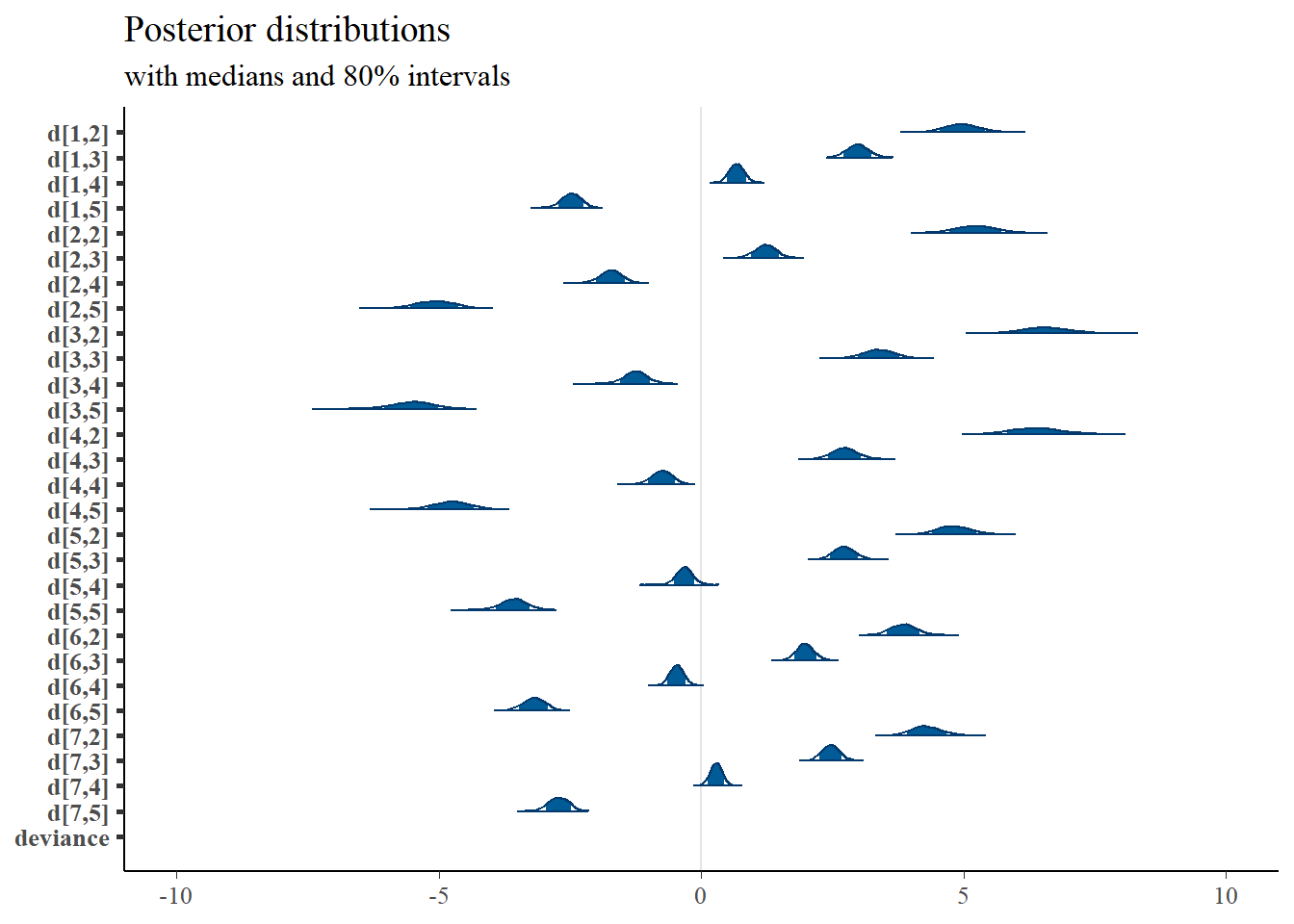

bayesplot::mcmc_areas(
  plot.data,
  pars = c(paste0("a[", 1:7, "]")),
  prob = 0.8) +
  plot_title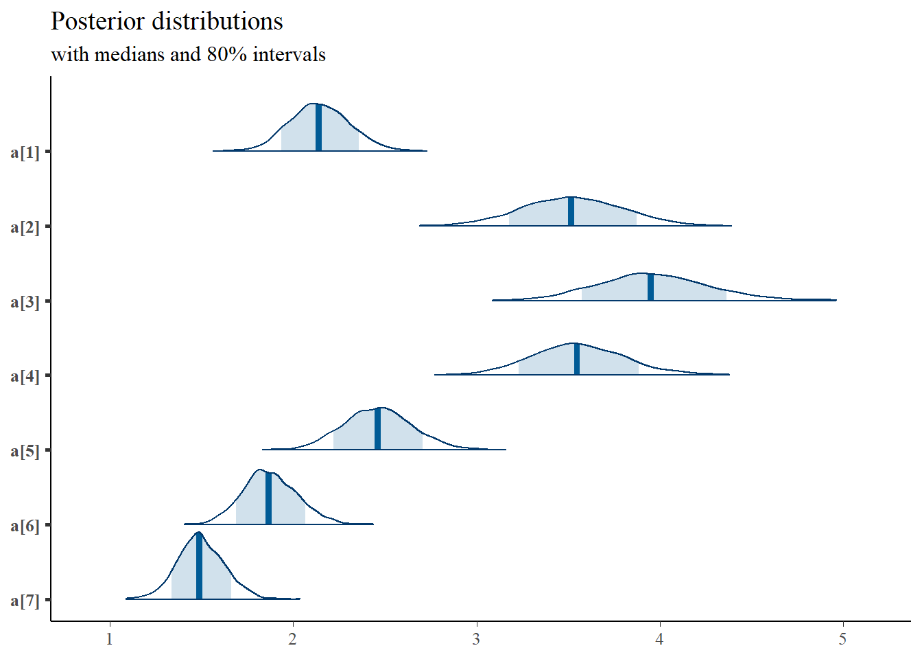

bayesplot::mcmc_acf(plot.data,pars = c(paste0("a[", 1:7, "]")))

bayesplot::mcmc_trace(plot.data,pars = c(paste0("a[", 1:7, "]")))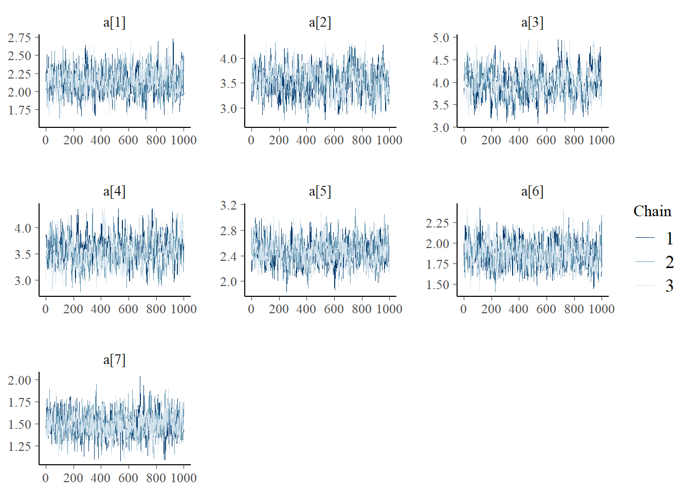

ggmcmc::ggs_grb(ggs(jags.mcmc), family="d")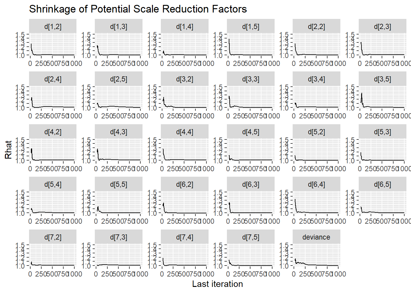

ggmcmc::ggs_grb(ggs(jags.mcmc), family="a")

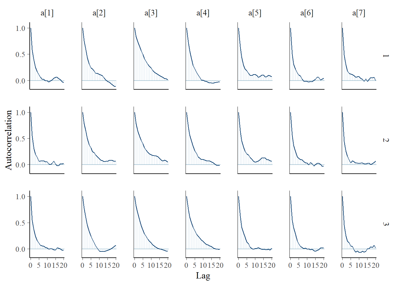
ggmcmc::ggs_autocorrelation(ggs(jags.mcmc), family="d")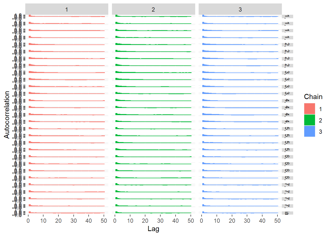

11.8 PI Example - Stan

model_irt_peer_int <- '
data {
  int  N;
  int  J;
  int  K;
  int  x[N,J];
}

parameters {
  real<lower=0> a[J]; //discrimination
  ordered[K-1] d[J]; //location/thresholds
  real theta[N]; //person parameters
}

model {
  // item response probabilities
  for(n in 1:N){
    for(j in 1:J){
      x[n,j] ~ ordered_logistic(a[j]*theta[n], d[j,1:(K-1)]);
    }
  }
  //measurement model priors
  theta ~ normal(0,1);
  for(j in 1:J){
    a[j] ~ normal(1,2)T[0,];
    d[j,1] ~ normal(-2,2);
    d[j,2] ~ normal(-1,2)T[d[j,1],];
    d[j,3] ~ normal(1,2)T[d[j,2],];
    d[j,4] ~ normal(2,2)T[d[j,3],];
  }
}

'


# initial values
start_values <- list(
  list(
    d= matrix(c(-3.00E+00, -1.00E+00, 0.00E+00, 1.00E+00,
               -3.00E+00, -1.00E+00, 0.00E+00, 1.00E+00,
               -3.00E+00, -1.00E+00, 0.00E+00, 1.00E+00,
               -3.00E+00, -1.00E+00, 0.00E+00, 1.00E+00,
               -3.00E+00, -1.00E+00, 0.00E+00, 1.00E+00,
               -3.00E+00, -1.00E+00, 0.00E+00, 1.00E+00,
               -3.00E+00, -1.00E+00, 0.00E+00, 1.00E+00),
      ncol=4, nrow=7, byrow=T),
    a=c(1.00E-01, 1.00E-01, 1.00E-01, 1.00E-01, 1.00E-01, 1.00E-01, 1.00E-01)),
  list(
    d= matrix(c(-2.00E+00, 0.00E+00, 1.00E+00, 2.00E+00,
               -2.00E+00, 0.00E+00, 1.00E+00, 2.00E+00,
               -2.00E+00, 0.00E+00, 1.00E+00, 2.00E+00,
               -2.00E+00, 0.00E+00, 1.00E+00, 2.00E+00,
               -2.00E+00, 0.00E+00, 1.00E+00, 2.00E+00,
               -2.00E+00, 0.00E+00, 1.00E+00, 2.00E+00,
               -2.00E+00, 0.00E+00, 1.00E+00, 2.00E+00),
      ncol=4, nrow=7, byrow=T),
    a=c(3.00E+00, 3.00E+00, 3.00E+00, 3.00E+00, 3.00E+00, 3.00E+00, 3.00E+00)),
  list(
    d= matrix(c(-1.00E+00, 1.00E+00, 2.00E+00, 3.00E+00,
               -1.00E+00, 1.00E+00, 2.00E+00, 3.00E+00,
               -1.00E+00, 1.00E+00, 2.00E+00, 3.00E+00,
               -1.00E+00, 1.00E+00, 2.00E+00, 3.00E+00,
               -1.00E+00, 1.00E+00, 2.00E+00, 3.00E+00,
               -1.00E+00, 1.00E+00, 2.00E+00, 3.00E+00,
               -1.00E+00, 1.00E+00, 2.00E+00, 3.00E+00),
              ncol=4, nrow=7, byrow=T),
    a=c(1.00E+00, 1.00E+00, 1.00E+00, 1.00E+00, 1.00E+00, 1.00E+00, 1.00E+00))
)

# dataset
dat <- read.table("data/PI.dat", header=T)

mydata <- list(
  N = nrow(dat),
  J = ncol(dat),
  K = 5,
  x = as.matrix(dat)
)


# Next, need to fit the model
#   I have explicitly outlined some common parameters
fit <- stan(
  model_code = model_irt_peer_int, # model code to be compiled
  data = mydata,          # my data
  init = start_values,    # starting values
  chains = 3,             # number of Markov chains
  warmup = 2000,          # number of warm up iterations per chain
  iter = 4000,            # total number of iterations per chain
  cores = 3,              # number of cores (could use one per chain)
  refresh = 0             # no progress shown
)

# first get a basic breakdown of the posteriors
print(fit,pars =c("d", "a", "theta[500]"))

## Inference for Stan model: anon_model.
## 3 chains, each with iter=4000; warmup=2000; thin=1; 
## post-warmup draws per chain=2000, total post-warmup draws=6000.
## 
##             mean se_mean   sd  2.5%   25%   50%   75% 97.5% n_eff Rhat
## d[1,1]     -5.07    0.01 0.36 -5.81 -5.30 -5.06 -4.83 -4.41  2523 1.00
## d[1,2]     -3.03    0.00 0.22 -3.46 -3.17 -3.02 -2.88 -2.62  2160 1.00
## d[1,3]     -0.71    0.00 0.15 -1.00 -0.80 -0.71 -0.60 -0.42  1307 1.00
## d[1,4]      2.47    0.00 0.20  2.10  2.33  2.46  2.60  2.86  1771 1.00
## d[2,1]     -5.51    0.01 0.41 -6.35 -5.77 -5.49 -5.22 -4.75  1577 1.00
## d[2,2]     -1.31    0.01 0.23 -1.77 -1.46 -1.30 -1.16 -0.88   984 1.01
## d[2,3]      1.76    0.01 0.24  1.30  1.60  1.75  1.91  2.24  1093 1.01
## d[2,4]      5.27    0.01 0.40  4.53  5.00  5.26  5.53  6.11  1668 1.00
## d[3,1]     -7.16    0.01 0.55 -8.29 -7.51 -7.15 -6.78 -6.13  1889 1.00
## d[3,2]     -3.70    0.01 0.35 -4.41 -3.93 -3.69 -3.47 -3.05  1322 1.00
## d[3,3]      1.30    0.01 0.26  0.81  1.12  1.30  1.48  1.81   873 1.01
## d[3,4]      5.90    0.01 0.48  5.01  5.56  5.88  6.21  6.90  2062 1.00
## d[4,1]     -6.74    0.01 0.50 -7.77 -7.07 -6.74 -6.40 -5.80  2066 1.00
## d[4,2]     -2.89    0.01 0.28 -3.45 -3.07 -2.89 -2.69 -2.37  1409 1.00
## d[4,3]      0.73    0.01 0.22  0.32  0.58  0.73  0.88  1.18   973 1.00
## d[4,4]      4.92    0.01 0.36  4.24  4.66  4.91  5.15  5.68  1897 1.00
## d[5,1]     -4.92    0.01 0.34 -5.61 -5.15 -4.92 -4.70 -4.30  2363 1.00
## d[5,2]     -2.79    0.01 0.22 -3.22 -2.93 -2.79 -2.64 -2.36  1793 1.00
## d[5,3]      0.29    0.00 0.16 -0.02  0.18  0.29  0.40  0.61  1186 1.00
## d[5,4]      3.58    0.01 0.26  3.10  3.41  3.58  3.76  4.10  2018 1.00
## d[6,1]     -3.89    0.01 0.26 -4.41 -4.06 -3.89 -3.71 -3.40  2385 1.00
## d[6,2]     -2.00    0.00 0.17 -2.34 -2.11 -2.00 -1.89 -1.68  1708 1.00
## d[6,3]      0.44    0.00 0.14  0.18  0.35  0.44  0.54  0.71  1306 1.00
## d[6,4]      3.17    0.00 0.22  2.76  3.02  3.16  3.31  3.61  2394 1.00
## d[7,1]     -4.35    0.00 0.30 -4.98 -4.55 -4.34 -4.14 -3.79  3967 1.00
## d[7,2]     -2.50    0.00 0.17 -2.84 -2.61 -2.50 -2.38 -2.16  2789 1.00
## d[7,3]     -0.31    0.00 0.12 -0.56 -0.39 -0.31 -0.23 -0.07  1818 1.00
## d[7,4]      2.70    0.00 0.19  2.35  2.58  2.70  2.83  3.08  2852 1.00
## a[1]        2.18    0.00 0.17  1.85  2.06  2.17  2.29  2.51  2316 1.00
## a[2]        3.73    0.01 0.29  3.19  3.53  3.72  3.91  4.33  1817 1.00
## a[3]        4.35    0.01 0.35  3.70  4.10  4.33  4.58  5.09  1924 1.00
## a[4]        3.74    0.01 0.29  3.21  3.55  3.73  3.93  4.33  1964 1.00
## a[5]        2.51    0.00 0.19  2.16  2.38  2.50  2.64  2.91  2262 1.00
## a[6]        1.88    0.00 0.15  1.61  1.78  1.88  1.97  2.19  2752 1.00
## a[7]        1.51    0.00 0.13  1.27  1.42  1.51  1.59  1.75  3207 1.00
## theta[500]  0.50    0.00 0.25  0.01  0.33  0.49  0.66  1.00  8485 1.00
## 
## Samples were drawn using NUTS(diag_e) at Mon Jul 25 08:34:57 2022.
## For each parameter, n_eff is a crude measure of effective sample size,
## and Rhat is the potential scale reduction factor on split chains (at 
## convergence, Rhat=1).

# plot the posterior in a
#  95% probability interval
#  and 80% to contrast the dispersion
plot(fit,pars =c("d", "a", "theta[500]"))

## ci_level: 0.8 (80% intervals)

## outer_level: 0.95 (95% intervals)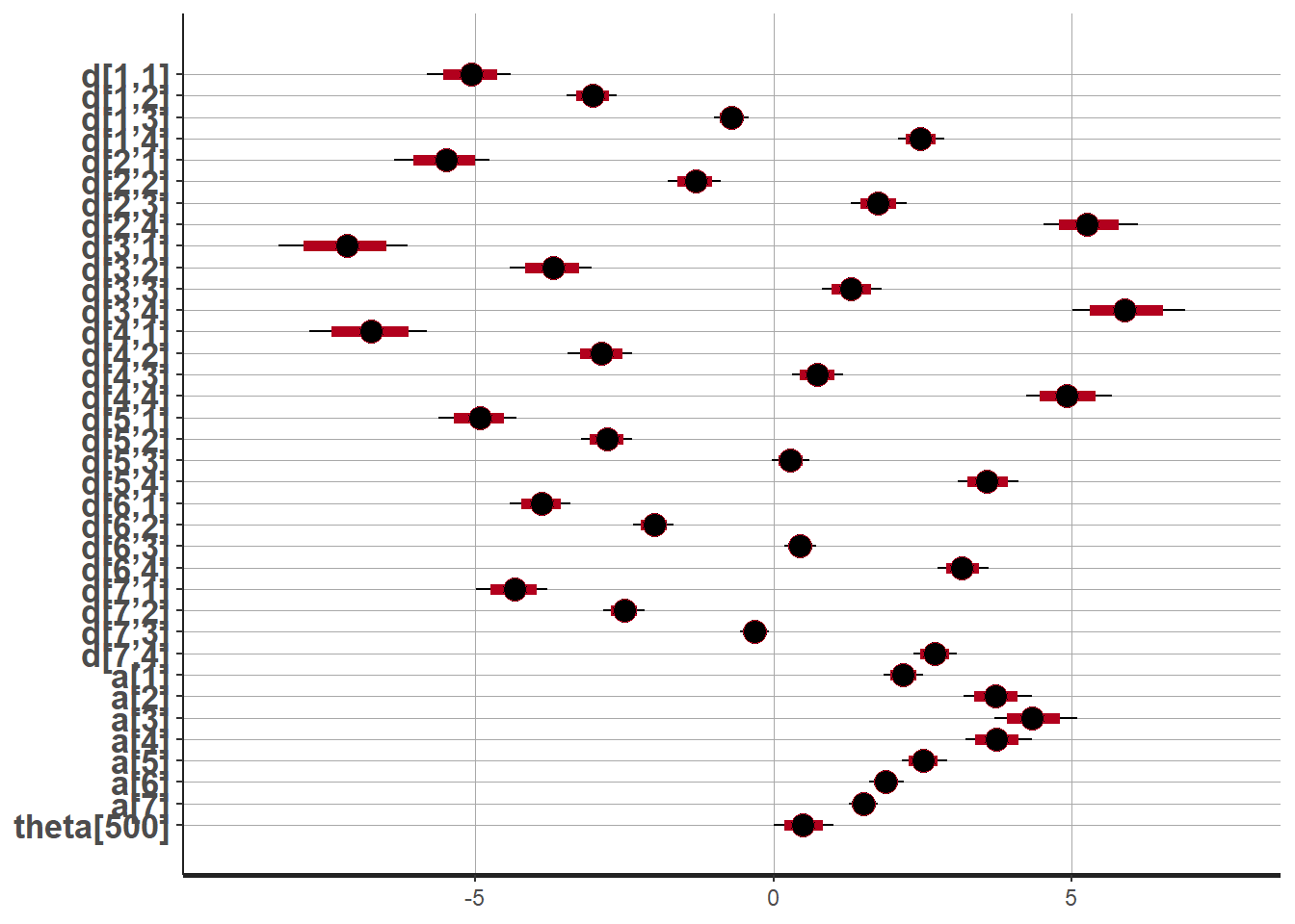

# traceplots
rstan::traceplot(fit,pars =c("d", "a", "theta[500]"), inc_warmup = TRUE)

# Gelman-Rubin-Brooks Convergence Criterion
ggs_grb(ggs(fit, family = c("d"))) +
   theme_bw() + theme(panel.grid = element_blank())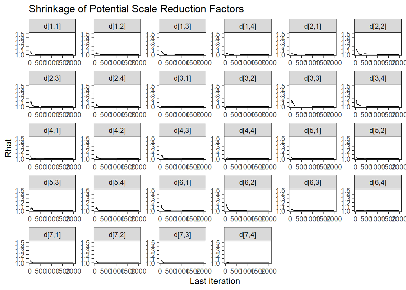

ggs_grb(ggs(fit, family = "a")) +
   theme_bw() + theme(panel.grid = element_blank())

ggs_grb(ggs(fit, family = "theta[500]")) +
   theme_bw() + theme(panel.grid = element_blank())

## Warning in max(D$Iteration): no non-missing arguments to max; returning -Inf

## Error in ggs_grb(ggs(fit, family = "theta[500]")): At least two chains are required

# autocorrelation
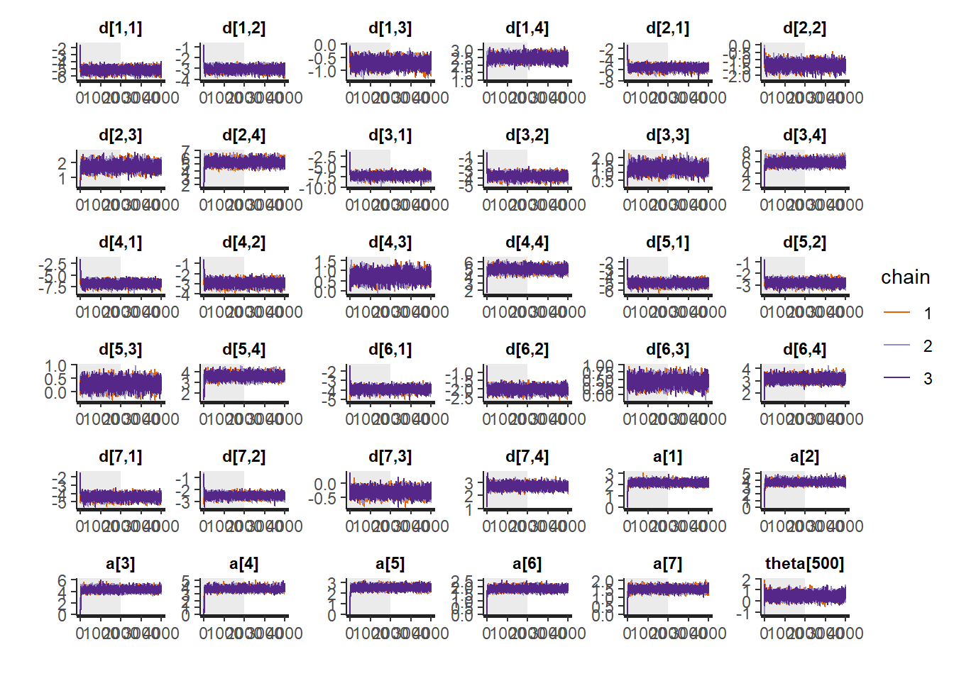
ggs_autocorrelation(ggs(fit, family="d")) +
   theme_bw() + theme(panel.grid = element_blank())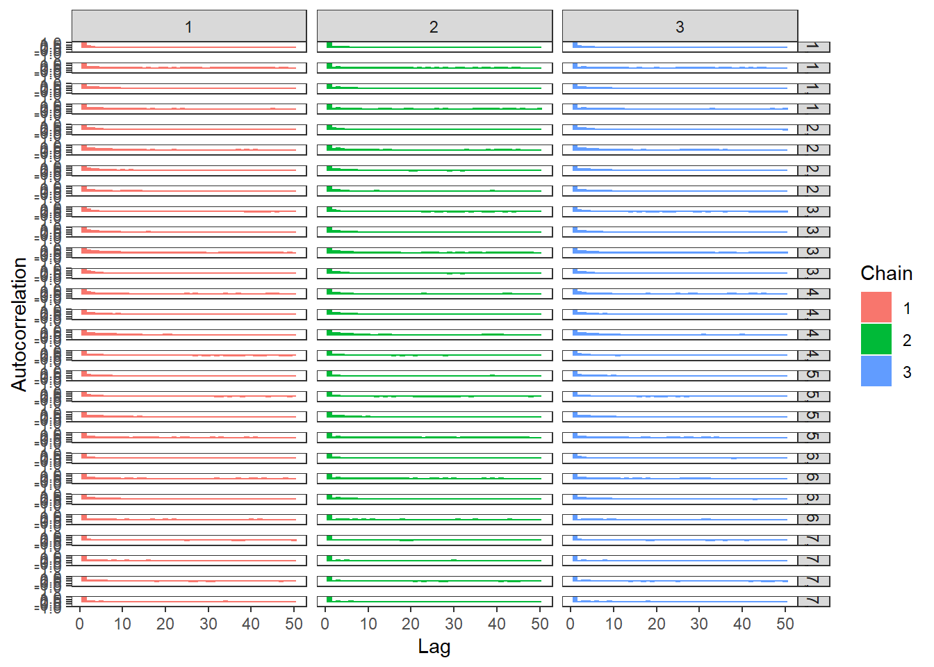

ggs_autocorrelation(ggs(fit, family="a")) +
   theme_bw() + theme(panel.grid = element_blank())

ggs_autocorrelation(ggs(fit, family="theta[500]")) +
   theme_bw() + theme(panel.grid = element_blank())

## Warning in max(D$Iteration): no non-missing arguments to max; returning -Inf

## Error in sprintf("nLags=%d is larger than number of iterations, computing until max possible lag %d", : invalid format '%d'; use format %f, %e, %g or %a for numeric objects

# plot the posterior density
plot.data <- as.matrix(fit)

mcmc_areas(plot.data, pars = paste0("d[1,",1:4,"]"),prob = 0.8)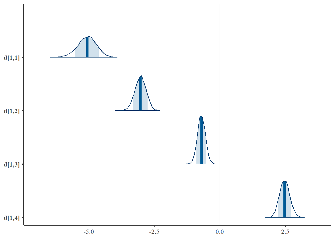

mcmc_areas(plot.data, pars = paste0("d[2,",1:4,"]"),prob = 0.8)

mcmc_areas(plot.data, pars = paste0("d[3,",1:4,"]"),prob = 0.8)

mcmc_areas(plot.data, pars = paste0("d[4,",1:4,"]"),prob = 0.8)

mcmc_areas(plot.data, pars = paste0("d[5,",1:4,"]"),prob = 0.8)

mcmc_areas(plot.data, pars = paste0("d[6,",1:4,"]"),prob = 0.8)

mcmc_areas(plot.data, pars = paste0("d[7,",1:4,"]"),prob = 0.8)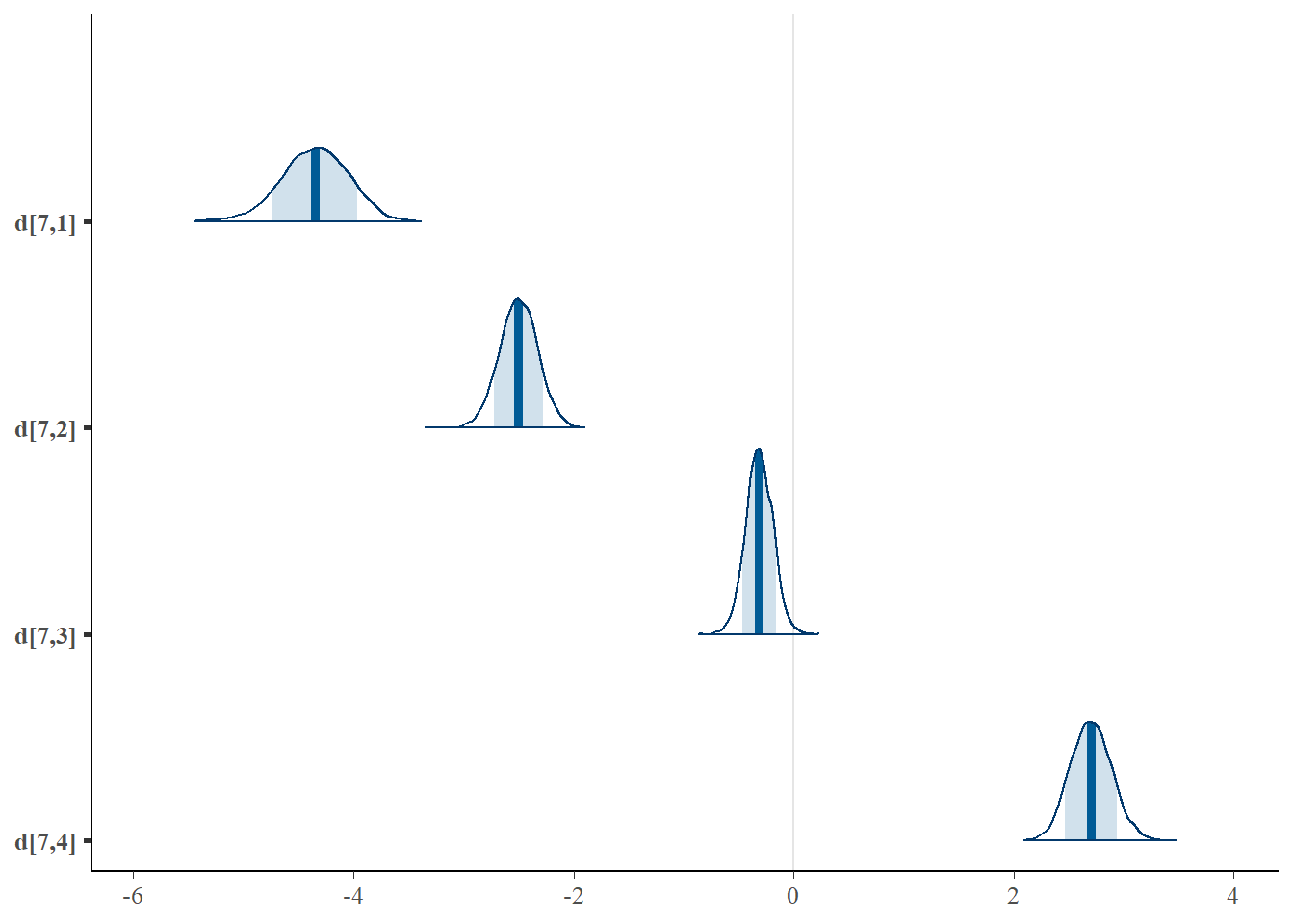

mcmc_areas(plot.data, pars = paste0("a[",1:7,"]"),prob = 0.8)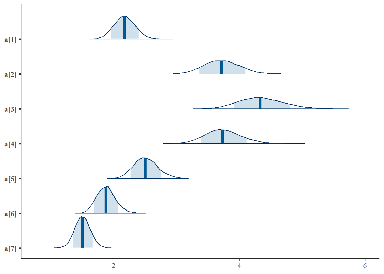

mcmc_areas(plot.data, pars = paste0("theta[500]"),prob = 0.8)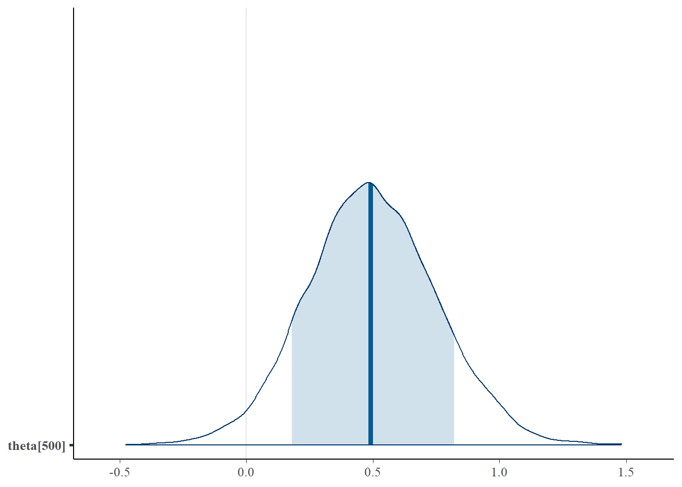

11.9 Latent Response Formulation

Connecting IRT models to a factor analytic perspective can be helpful from a modeling standpoint. Especially when one’s model is multidimensional leading into structural equation models. A useful connection can be made by introducing extra variable(s) into the model to represent the latent response variable underlying the observed categorical response variable. We can think of this latent response variables as

• a latent continuous variable hypothesized to underlie the observed categorical variable that discretized due to data collection or difficulty in measurement; or

• when this natural interpretation is not appropriate, we can think of the latent response variable as a propensity measure for the given response. Although this is not a perfect interpretation, the use of a latent response formulation eases some of the computational machinery and allows for a nice connection between IRT and CFA models.

Next, the latent response formulation is shown for a set of dichotomous outcomes. This model is conceptually a 2-PL/2-PNO (2 parameter normal ogive) model and is essentially a probit model. The model can be defined as

\[x^{\ast}_{ij} = a_j\theta_i+d_j+\varepsilon_{ij},\]

where, an important feature is how this latent response is related back to the observed indicator. The range of possible values of a latent response is defined conditional on the value of the observed response. That is, \[ x^{\ast}_{ij} \sim \cases{ N(a_j\theta_i+d_j, 1)I(x^{\ast}_{ij}\geq0)\ \ \ \ if\ x=1\\ N(a_j\theta_i+d_j, 1)I(x^{\ast}_{ij}<0)\ \ \ \ if\ x=0} \]

11.9.1 A Comment on use of JAGS

After a lot of trial and error in JAGS, I discovered that the model for a latent response is a bit difficult to code up as defined above. I found a way to utilize the idea of the latent response formulation. The approach is not perfect and better ways of coding the model are likely more efficient.

In the approached below, which I demonstrate in the example code below, I utilize the model nearly identically to the above specification. However, I alter the model so that an “observed stochastic node” can be utilized as part of the sampling. That is, I had to use the latent response variables to obtain a probability of the observed response. This is straightforward as the latent response variable is based on the normal standard normal distribution and we can use the cumulative normal distribution CDF (Phi) to obtain a probability that represents the probability of responding “1”. Then a Bernoulli distribution is used as the data model. This approach is a straightforward addition to the latent response modeling and connects well to what is done in IRT models above.

11.9.2 LSAT Example Revisted - JAGS

jags.model.lsat <- function(){

for (i in 1:n){
  for(j in 1:J){
    # latent response variable
    
    xpos[i,j] ~ dnorm(0, 1);T(0,)
    xneg[i,j] ~ dnorm(0, 1);T(,0)
    
    mu[i,j] = xpos[i,j]*z[i,j] + xneg[i,j]*(1-z[i,j])
    
    # compute probabilities based on probit to obtain probabilities for observed categories
    x[i,j] ~ dbern(phi(xstar[i,j] - d[j]))

  }
  
  xstar[i,1:J] ~ dmnorm.vcov(mu[i,1:J], Omega)
  
  
}

psi ~ dgamma(1, 0.5)
invpsi = 1/psi;
for(i in 1:n){
  theta[i] ~ dnorm(0, invpsi)  # distribution for the latent variables
}

for(j in 1:J){
  d[j] ~ dnorm(0, .5)          # Locations for observables
}
a[1] = 1
for(j in 2:J){
  a[j] ~ dnorm(1, .5)    # Discriminations for observables
}

for(i in 1:J){
  for(j in 1:J){
    Omega[i,j] = ifelse(i==j, 1 + psi*a[i]*a[j], psi*a[i]*a[j])
  }
}


} # closes the model

# initial values
start_values <- list(
  list("d"=c(1.00, 1.00, 1.00, 1.00, 1.00),
       "a"=c(NA, 1.00, 1.00, 1.00, 1.00)),
  list("d"=c(-3.00, -3.00, -3.00, -3.00, -3.00),
       "a"=c(NA, 3.00, 3.00, 3.00, 3.00)),
  list("d"=c(3.00, 3.00, 3.00, 3.00, 3.00),
       "a"=c(NA, 0.1, 0.1, 0.1, 0.1))
)

# vector of all parameters to save
param_save <- c("a", "d", "theta", "psi", "Omega", "xstar")

# dataset
dat <- read.table("data/LSAT.dat", header=T)

mydata <- list(
  n = nrow(dat),
  J = ncol(dat),
  x = as.matrix(dat),
  z = as.matrix(dat)
)

# fit model
fit <- jags(
  model.file=jags.model.lsat,
  data=mydata,
  inits=start_values,
  parameters.to.save = param_save,
  n.iter=2000,
  n.burnin = 1000,
  n.chains = 3,
  progress.bar = "none")

## Compiling model graph
##    Resolving undeclared variables
##    Allocating nodes
## Graph information:
##    Observed stochastic nodes: 5000
##    Unobserved stochastic nodes: 12010
##    Total graph size: 53123
## 
## Initializing model

#print(fit)
round(fit$BUGSoutput$summary[ !c(rownames(fit$BUGSoutput$summary) %like% "theta" |
                                   rownames(fit$BUGSoutput$summary) %like% "xstar" ), ], 3)

##                mean     sd     2.5%      25%      50%      75%    97.5%  Rhat n.eff
## Omega[1,1]    1.006  0.008    1.000    1.001    1.003    1.007    1.030 1.013  1500
## Omega[2,1]    0.003  0.007   -0.007    0.000    0.001    0.005    0.021 1.001  3000
## Omega[3,1]    0.003  0.007   -0.008    0.000    0.001    0.004    0.019 1.015   250
## Omega[4,1]    0.003  0.007   -0.010    0.000    0.001    0.005    0.020 1.009   280
## Omega[5,1]    0.003  0.008   -0.012    0.000    0.001    0.005    0.023 1.003  3000
## Omega[1,2]    0.003  0.007   -0.007    0.000    0.001    0.005    0.021 1.001  3000
## Omega[2,2]    1.006  0.009    1.000    1.000    1.002    1.007    1.032 1.003  3000
## Omega[3,2]    0.002  0.006   -0.008    0.000    0.000    0.003    0.019 1.009   570
## Omega[4,2]    0.002  0.006   -0.010   -0.001    0.000    0.003    0.018 1.001  3000
## Omega[5,2]    0.002  0.008   -0.010   -0.001    0.000    0.003    0.022 1.002  1900
## Omega[1,3]    0.003  0.007   -0.008    0.000    0.001    0.004    0.019 1.015   250
## Omega[2,3]    0.002  0.006   -0.008    0.000    0.000    0.003    0.019 1.009   570
## Omega[3,3]    1.005  0.009    1.000    1.000    1.002    1.007    1.031 1.047   230
## Omega[4,3]    0.002  0.007   -0.009    0.000    0.000    0.003    0.018 1.021   470
## Omega[5,3]    0.002  0.007   -0.010   -0.001    0.000    0.003    0.020 1.009  3000
## Omega[1,4]    0.003  0.007   -0.010    0.000    0.001    0.005    0.020 1.009   280
## Omega[2,4]    0.002  0.006   -0.010   -0.001    0.000    0.003    0.018 1.001  3000
## Omega[3,4]    0.002  0.007   -0.009    0.000    0.000    0.003    0.018 1.021   470
## Omega[4,4]    1.006  0.010    1.000    1.000    1.002    1.007    1.037 1.004  2100
## Omega[5,4]    0.002  0.008   -0.010   -0.001    0.000    0.003    0.023 1.009  1500
## Omega[1,5]    0.003  0.008   -0.012    0.000    0.001    0.005    0.023 1.003  3000
## Omega[2,5]    0.002  0.008   -0.010   -0.001    0.000    0.003    0.022 1.002  1900
## Omega[3,5]    0.002  0.007   -0.010   -0.001    0.000    0.003    0.020 1.009  3000
## Omega[4,5]    0.002  0.008   -0.010   -0.001    0.000    0.003    0.023 1.009  1500
## Omega[5,5]    1.007  0.013    1.000    1.000    1.002    1.008    1.042 1.002  1900
## a[1]          1.000  0.000    1.000    1.000    1.000    1.000    1.000 1.000     1
## a[2]          0.779  1.144   -1.331    0.014    0.695    1.490    3.275 1.005   530
## a[3]          0.722  1.100   -1.318   -0.009    0.658    1.418    3.058 1.001  3000
## a[4]          0.760  1.138   -1.374    0.013    0.709    1.480    3.115 1.003  1400
## a[5]          0.713  1.183   -1.586   -0.084    0.727    1.499    3.023 1.001  2400
## d[1]         -1.786  0.105   -1.994   -1.856   -1.783   -1.715   -1.586 1.009   230
## d[2]         -0.664  0.075   -0.812   -0.715   -0.664   -0.613   -0.521 1.008   390
## d[3]         -0.162  0.069   -0.300   -0.208   -0.161   -0.116   -0.027 1.007   310
## d[4]         -0.875  0.073   -1.024   -0.923   -0.872   -0.824   -0.737 1.015   140
## d[5]         -1.397  0.084   -1.562   -1.450   -1.398   -1.340   -1.231 1.001  2500
## deviance   1874.048 44.526 1787.777 1844.505 1873.781 1903.707 1963.353 1.038    59
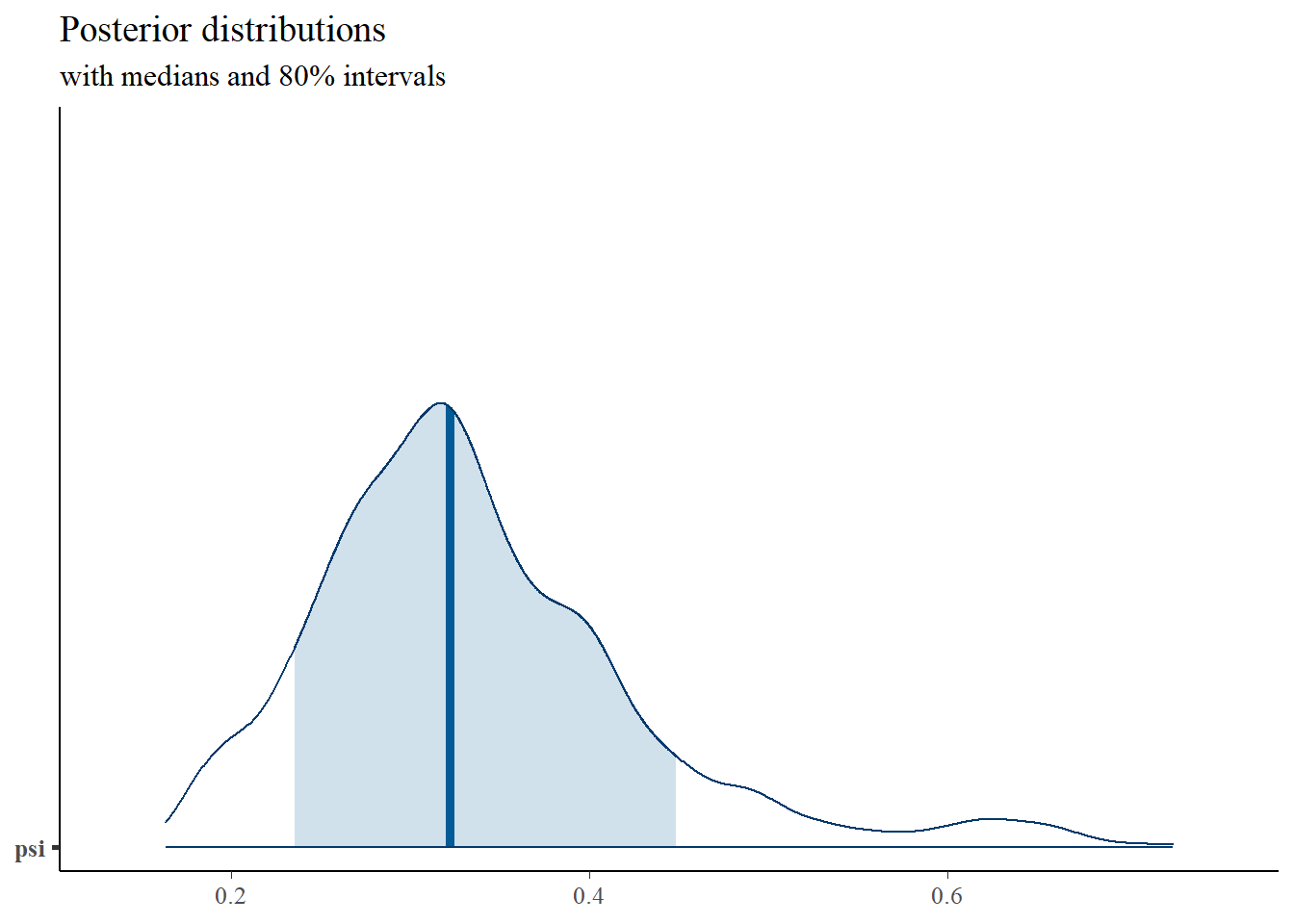
## psi           0.006  0.008    0.000    0.001    0.003    0.007    0.030 1.005   440

round(fit$BUGSoutput$summary[c("xstar[4,4]","xstar[4,5]","xstar[10,4]","xstar[10,5]"),] ,3)

##               mean    sd   2.5%    25%    50%    75%  97.5%  Rhat n.eff
## xstar[4,4]  -1.502 0.948 -3.426 -2.145 -1.453 -0.829  0.179 1.031    71
## xstar[4,5]   0.863 1.117 -1.072  0.089  0.769  1.537  3.274 1.012   280
## xstar[10,4]  1.052 1.087 -0.838  0.320  0.987  1.675  3.501 1.005   470
## xstar[10,5] -1.880 1.002 -4.120 -2.459 -1.772 -1.185 -0.126 1.018   200

# extract posteriors for all chains
jags.mcmc <- as.mcmc(fit)
# the below two plots are too big to be useful given the 1000 observations.
#R2jags::traceplot(jags.mcmc)

# gelman-rubin-brook
#gelman.plot(jags.mcmc)

# convert to single data.frame for density plot
a <- colnames(as.data.frame(jags.mcmc[[1]]))
plot.data <- data.frame(as.matrix(jags.mcmc, chains=T, iters = T))
colnames(plot.data) <- c("chain", "iter", a)


plot_title <- ggtitle("Posterior distributions",
                      "with medians and 80% intervals")
mcmc_areas(
  plot.data,
  pars = c(paste0("d[",1:5,"]")),
  prob = 0.8) +
  plot_title

mcmc_areas(
  plot.data,
  pars = c(paste0("a[", 2:5, "]")),
  prob = 0.8) +
  plot_title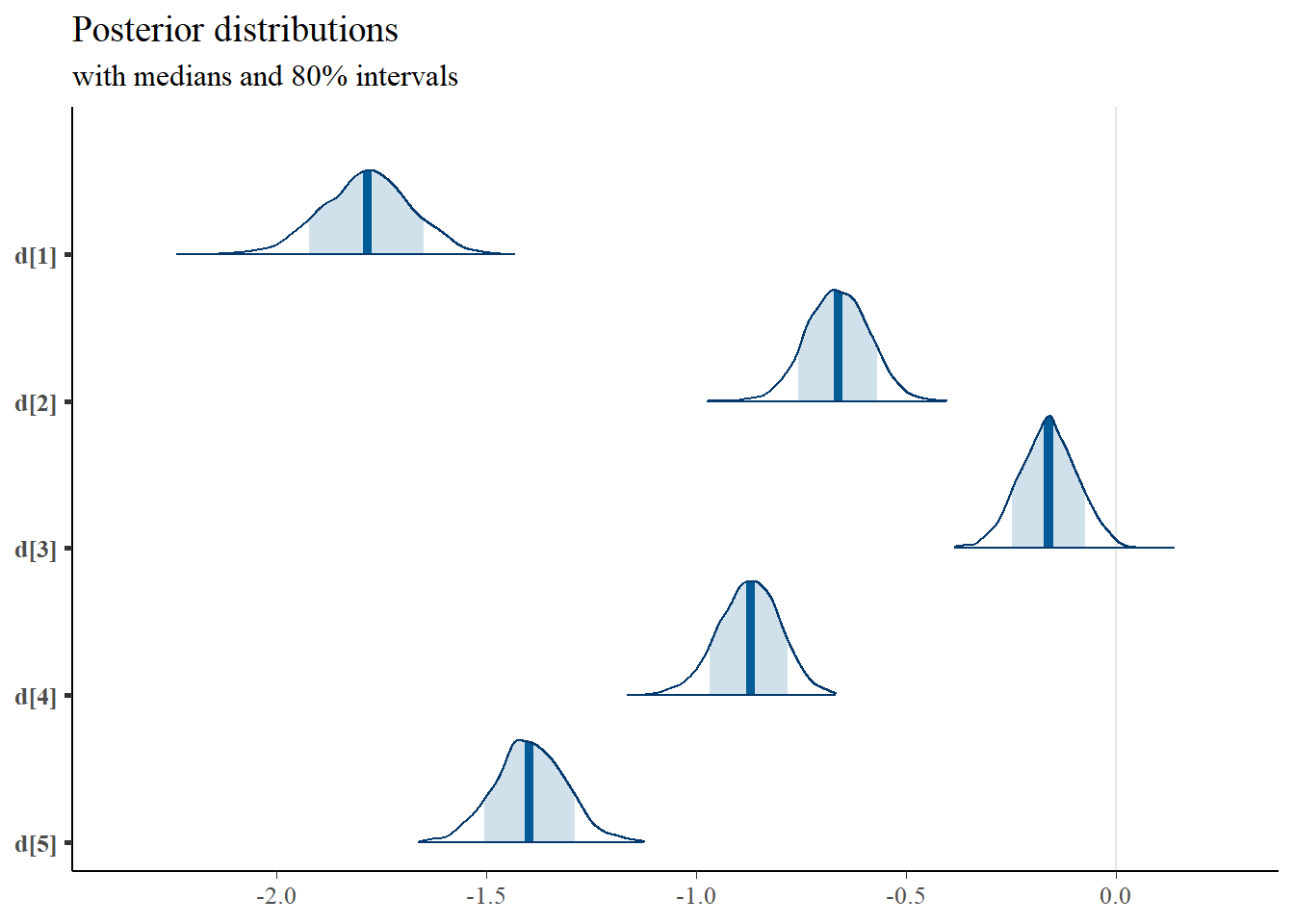

print(mydata$x[50,])

## Item.1 Item.2 Item.3 Item.4 Item.5 
##      0      1      0      1      1

mcmc_areas(
  plot.data,
  pars = c("xstar[50,1]", "xstar[50,2]"),
  prob = 0.8) +
  plot_title

11.9.3 LSAT Example Revisted - Stan

model_lrv <- [2597 chars quoted with ''']
cat(model_lrv)

## 
## functions {
##   //x = data vector of 1,2,...,nlevs to determine which nu to use
##   //mu=vector of K means fixed to 0 to align with blavaan
##   //L= cholesky  factor for K variables
##   //b=vector of bounds/threshold values
##   //u=vector of random uniform numbers (K)
##   vector[] tmvn(int[] y, vector mu, matrix L, vector b, real[] u) {
##     int K = rows(mu);
##     vector[K] d;
##     vector[K] z;
##     vector[K] out[2];
##     for (k in 1:K) {
##       int km1 = k - 1;
##       real nu;
##       //y==0 => upper bound only
##       if (y[k] == 0) {
##         real z_star = (b[k] - (mu[k] + ((k > 1) ? L[k,1:km1] * head(z, km1) : 0))) /  L[k,k];
##         real u_star = Phi(z_star); //normal CDF for implied density of TMVN
##         nu = u_star * u[k];
##         d[k] = u_star;
##       }
##       //y==1 => lower bound only
##       if(y[k] == 1) {
##         real z_star = (b[k] - (mu[k] + ((k > 1) ? L[k,1:km1] * head(z, km1) : 0))) /  L[k,k];
##         real u_star = Phi(z_star);
##         d[k] = 1 - u_star;
##         nu = u_star + d[k] * u[k];
##       }
##       z[k] = inv_Phi(nu); //convert back to z-score from uniform variate
##     }
## 
##     out[1] = z; //simulated ystar value
##     out[2] = d; //density
##     return(out);
##   }
## 
## }
## data {
##   int<lower=1>  N;
##   int<lower=1>  J;
##   array[N, J] int<lower=0, upper=1> x;
## }
## 
## parameters {
##   vector[J] tau; //threshold parameters
##   vector[J-1] lambda_fr; //factor loadings
##   real<lower=0> psi; // factor standard deviation
##   real eta[N]; //factor scores
##   array[N, J] real<lower=0, upper=1> u; // nuisance that absorbs inequality constraints
## }
## 
## transformed parameters {
##   vector[J] lambda;
##   matrix[J,J] Omega;
##   matrix[J,J] L_Omega;
##   real psi_var;
## 
##   lambda[1] = 1;
##   lambda[2:J] = lambda_fr;
##   psi_var = psi^2;
## 
##   for(d in 1:J){
##     for(f in 1:J){
##       if(d==f){
##         Omega[d,f] = 1 + psi_var*lambda[d]^2;
##       } else {
##         Omega[d,f] = psi_var*lambda[d]*lambda[f];
##       }
##     }
##   }
##   //decomponse for use in stan sampling statement
##   L_Omega = cholesky_decompose(Omega);
## }
## 
## model {
##   for(n in 1:N)
##     target += log(tmvn(x[n,1:J], rep_vector(0,J), L_Omega, tau, u[n,1:J])[2]);
##   // Jacobian adjustments to kernal density for use of TMVN density on x*
##   // implicit: u ~ uniform(0,1)
##   // truncated multivariate normal
##   
##   
##   //priors for measurement model
##   psi ~ gamma(1, 0.5);
##   eta ~ normal(0,psi);
##   lambda_fr ~ normal(0,1.5);
##   tau ~ normal(0,1.5);
## }
## 
## generated quantities {
##   corr_matrix[J] Omega_cor;
## 
##   for(d in 1:J){
##     for(f in 1:J){
##       if(d==f){
##         Omega_cor[d,f] = 1;
##       } else {
##         Omega_cor[d,f] = Omega[d,f]/(sqrt(Omega[d,d])*sqrt(Omega[f,f]));
##       }
##     }
##   }
## }

# initial values
start_values <- list(
  list("tau"=c(1.00, 1.00, 1.00, 1.00, 1.00),
       "lambda_fr"=c(1.00, 1.00, 1.00, 1.00)),
  list("tau"=c(-3.00, -3.00, -3.00, -3.00, -3.00),
       "lambda_fr"=c(3.00, 3.00, 3.00, 3.00)),
  list("tau"=c(3.00, 3.00, 3.00, 3.00, 3.00),
       "lambda_fr"=c(0.1, 0.1, 0.1, 0.1))
)

# dataset
dat <- read.table("data/LSAT.dat", header=T)

mydata <- list(
  N = nrow(dat),
  J = ncol(dat),
  x = as.matrix(dat)
)


# Next, need to fit the model
#   I have explicitly outlined some common parameters
fit <- stan(
  model_code = model_lrv, # model code to be compiled
  data = mydata,          # my data
  #init = start_values,    # starting values
  chains = 4,             # number of Markov chains
  warmup = 1000,          # number of warm up iterations per chain
  iter = 2000,            # total number of iterations per chain
  cores = 4,              # number of cores (could use one per chain)
  refresh = 0             # no progress shown
)

## Warning: There were 111 transitions after warmup that exceeded the maximum treedepth. Increase max_treedepth above 10. See
## https://mc-stan.org/misc/warnings.html#maximum-treedepth-exceeded

## Warning: There were 4 chains where the estimated Bayesian Fraction of Missing Information was low. See
## https://mc-stan.org/misc/warnings.html#bfmi-low

## Warning: Examine the pairs() plot to diagnose sampling problems

## Warning: The largest R-hat is NA, indicating chains have not mixed.
## Running the chains for more iterations may help. See
## https://mc-stan.org/misc/warnings.html#r-hat

## Warning: Bulk Effective Samples Size (ESS) is too low, indicating posterior means and medians may be unreliable.
## Running the chains for more iterations may help. See
## https://mc-stan.org/misc/warnings.html#bulk-ess

## Warning: Tail Effective Samples Size (ESS) is too low, indicating posterior variances and tail quantiles may be unreliable.
## Running the chains for more iterations may help. See
## https://mc-stan.org/misc/warnings.html#tail-ess

# first get a basic breakdown of the posteriors
print(fit,pars =c("lambda", "tau","psi", "Omega_cor"))

## Inference for Stan model: anon_model.
## 4 chains, each with iter=2000; warmup=1000; thin=1; 
## post-warmup draws per chain=1000, total post-warmup draws=4000.
## 
##                 mean se_mean   sd  2.5%   25%   50%   75% 97.5% n_eff Rhat
## lambda[1]       1.00     NaN 0.00  1.00  1.00  1.00  1.00  1.00   NaN  NaN
## lambda[2]       1.36    0.08 0.50  0.58  1.00  1.29  1.64  2.55    39 1.09
## lambda[3]       1.64    0.08 0.57  0.77  1.23  1.55  1.96  3.02    55 1.07
## lambda[4]       1.28    0.09 0.49  0.53  0.94  1.21  1.56  2.44    31 1.11
## lambda[5]       1.15    0.07 0.49  0.39  0.80  1.08  1.43  2.28    54 1.08
## tau[1]         -1.52    0.01 0.08 -1.68 -1.56 -1.51 -1.46 -1.38    56 1.07
## tau[2]         -0.60    0.00 0.05 -0.71 -0.64 -0.60 -0.57 -0.50  3383 1.00
## tau[3]         -0.15    0.00 0.05 -0.24 -0.18 -0.15 -0.12 -0.06  5483 1.00
## tau[4]         -0.77    0.00 0.06 -0.89 -0.81 -0.77 -0.74 -0.67  2969 1.00
## tau[5]         -1.20    0.00 0.07 -1.36 -1.24 -1.20 -1.16 -1.08  2196 1.00
## psi             0.34    0.02 0.09  0.19  0.28  0.32  0.38  0.61    14 1.27
## Omega_cor[1,1]  1.00     NaN 0.00  1.00  1.00  1.00  1.00  1.00   NaN  NaN
## Omega_cor[1,2]  0.12    0.01 0.04  0.06  0.09  0.12  0.15  0.22    29 1.12
## Omega_cor[1,3]  0.14    0.01 0.05  0.07  0.11  0.14  0.17  0.26    21 1.16
## Omega_cor[1,4]  0.12    0.01 0.04  0.05  0.09  0.11  0.14  0.20    40 1.10
## Omega_cor[1,5]  0.10    0.01 0.04  0.04  0.08  0.10  0.13  0.19    57 1.07
## Omega_cor[2,1]  0.12    0.01 0.04  0.06  0.09  0.12  0.15  0.22    29 1.12
## Omega_cor[2,2]  1.00     NaN 0.00  1.00  1.00  1.00  1.00  1.00   NaN  NaN
## Omega_cor[2,3]  0.17    0.00 0.05  0.08  0.14  0.17  0.21  0.27  1647 1.01
## Omega_cor[2,4]  0.14    0.00 0.04  0.07  0.11  0.14  0.17  0.23  2857 1.00
## Omega_cor[2,5]  0.13    0.00 0.05  0.05  0.09  0.13  0.16  0.23  1912 1.00
## Omega_cor[3,1]  0.14    0.01 0.05  0.07  0.11  0.14  0.17  0.26    21 1.16
## Omega_cor[3,2]  0.17    0.00 0.05  0.08  0.14  0.17  0.21  0.27  1647 1.01
## Omega_cor[3,3]  1.00     NaN 0.00  1.00  1.00  1.00  1.00  1.00   NaN  NaN
## Omega_cor[3,4]  0.17    0.00 0.05  0.08  0.13  0.17  0.20  0.26  1953 1.00
## Omega_cor[3,5]  0.15    0.00 0.05  0.07  0.12  0.15  0.18  0.24  2782 1.00
## Omega_cor[4,1]  0.12    0.01 0.04  0.05  0.09  0.11  0.14  0.20    40 1.10
## Omega_cor[4,2]  0.14    0.00 0.04  0.07  0.11  0.14  0.17  0.23  2857 1.00
## Omega_cor[4,3]  0.17    0.00 0.05  0.08  0.13  0.17  0.20  0.26  1953 1.00
## Omega_cor[4,4]  1.00     NaN 0.00  1.00  1.00  1.00  1.00  1.00   NaN  NaN
## Omega_cor[4,5]  0.12    0.00 0.05  0.04  0.09  0.12  0.15  0.22  1948 1.00
## Omega_cor[5,1]  0.10    0.01 0.04  0.04  0.08  0.10  0.13  0.19    57 1.07
## Omega_cor[5,2]  0.13    0.00 0.05  0.05  0.09  0.13  0.16  0.23  1912 1.00
## Omega_cor[5,3]  0.15    0.00 0.05  0.07  0.12  0.15  0.18  0.24  2782 1.00
## Omega_cor[5,4]  0.12    0.00 0.05  0.04  0.09  0.12  0.15  0.22  1948 1.00
## Omega_cor[5,5]  1.00     NaN 0.00  1.00  1.00  1.00  1.00  1.00   NaN  NaN
## 
## Samples were drawn using NUTS(diag_e) at Sun Jul 17 16:59:09 2022.
## For each parameter, n_eff is a crude measure of effective sample size,
## and Rhat is the potential scale reduction factor on split chains (at 
## convergence, Rhat=1).

rstan::traceplot(fit,pars =c("lambda_fr", "tau", "psi"), inc_warmup = TRUE)

# Gelman-Rubin-Brooks Convergence Criterion
ggs_grb(ggs(fit, family = c("lambda_fr"))) +
   theme_bw() + theme(panel.grid = element_blank())

ggs_grb(ggs(fit, family = "tau")) +
   theme_bw() + theme(panel.grid = element_blank())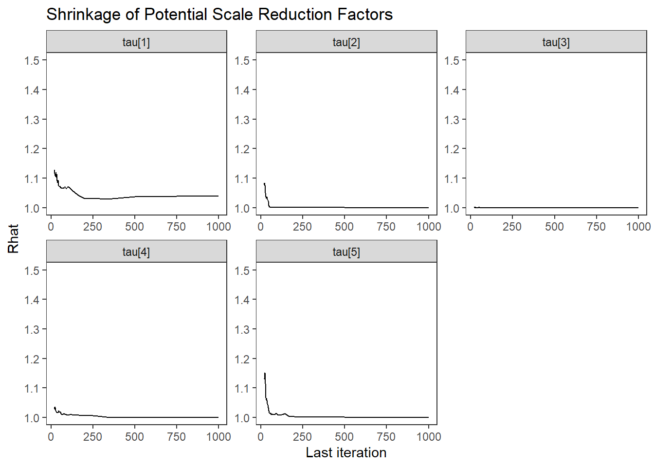

ggs_grb(ggs(fit, family = "psi")) +
   theme_bw() + theme(panel.grid = element_blank())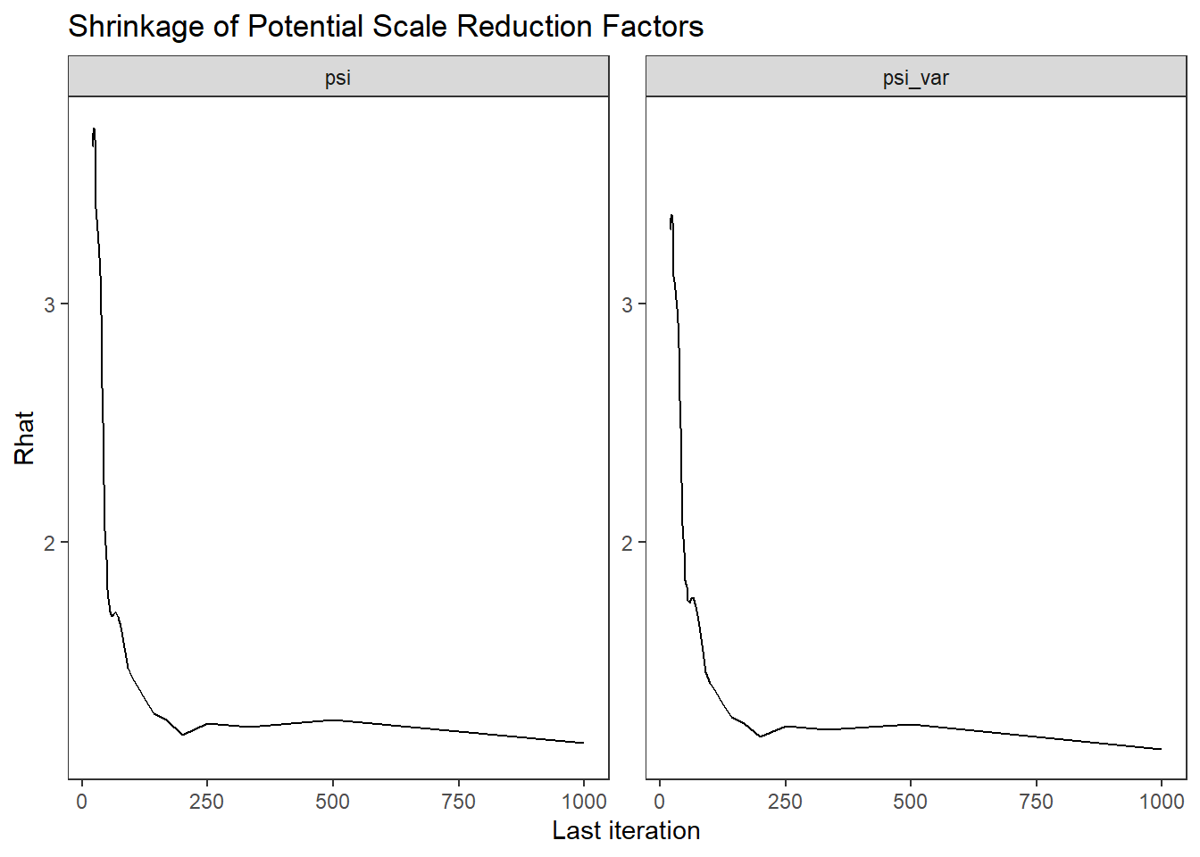

# autocorrelation
ggs_autocorrelation(ggs(fit, family="lambda_fr")) +
   theme_bw() + theme(panel.grid = element_blank())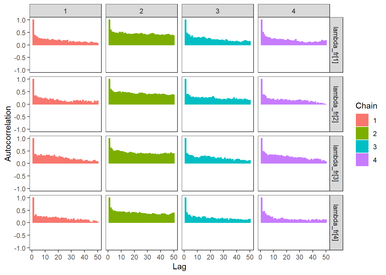

ggs_autocorrelation(ggs(fit, family="tau")) +
   theme_bw() + theme(panel.grid = element_blank())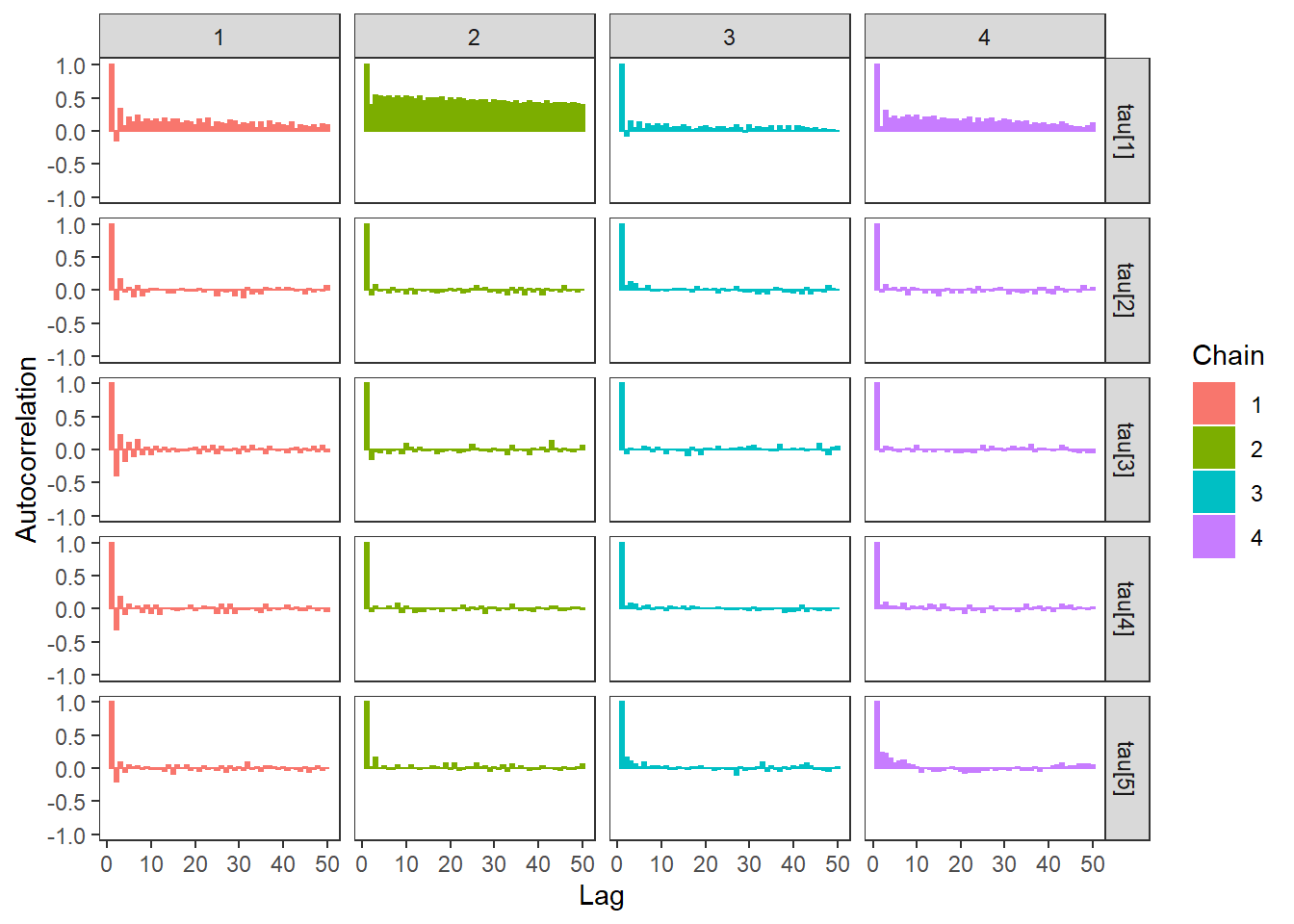

ggs_autocorrelation(ggs(fit, family="psi")) +
   theme_bw() + theme(panel.grid = element_blank())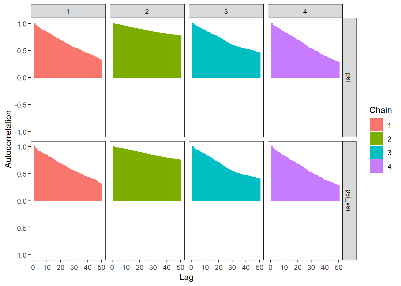

# plot the posterior density
plot.data <- as.matrix(fit)

plot_title <- ggtitle("Posterior distributions",
                      "with medians and 80% intervals")
mcmc_areas(
  plot.data,
  pars = paste0("lambda_fr[",1:4,"]"),
  prob = 0.8) +
  plot_title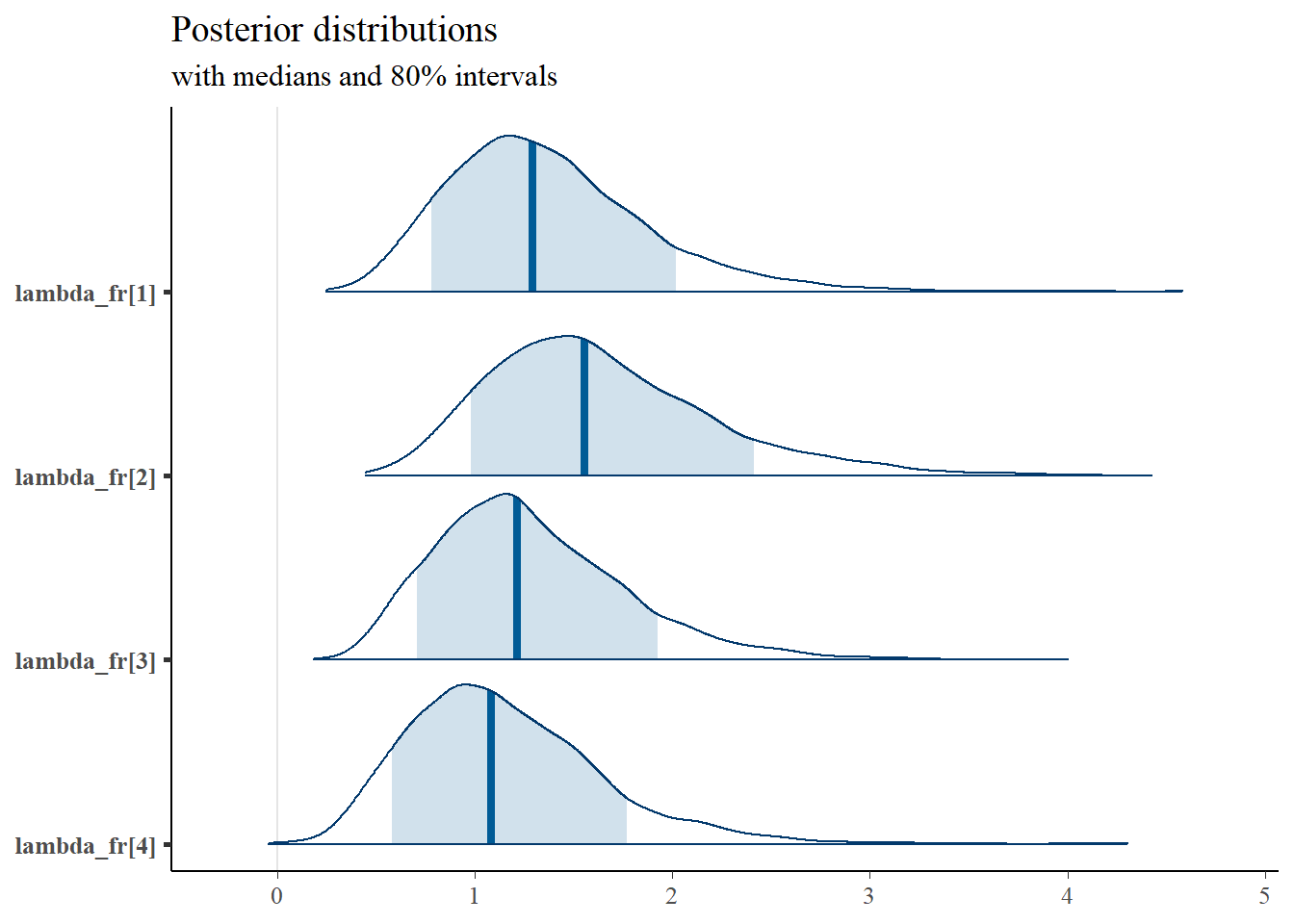

mcmc_areas(
  plot.data,
  pars = paste0("tau[",1:5,"]"),
  prob = 0.8) +
  plot_title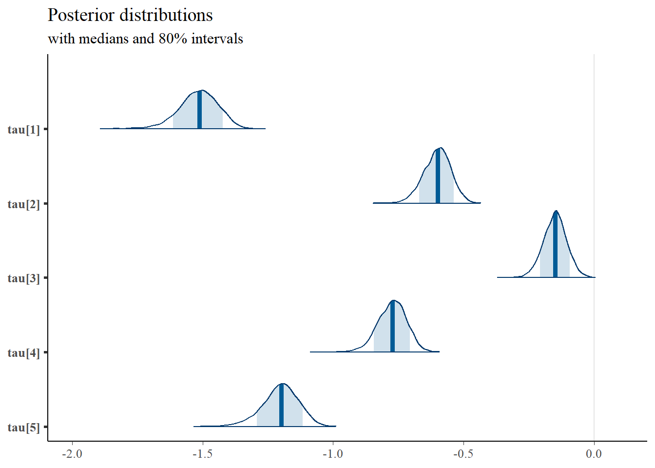

mcmc_areas(
  plot.data,
  pars = c("psi"),
  prob = 0.8) +
  plot_title

11.10 Final Notes

• A fully Bayesian approach to psychometric modeling helps highlight the major similarities between factor analytic frameworks and the item response theory perspective.