10 Model Evaluation
The goal of evaluating the model is to determine if the inferences suggested by the model are reasonable based one’s content area knowledge. The text and (BDA3) say that this evaluation of reasonableness is really a form of prior, that is “Gelman et al. (2013) argued tha when analysts deem that the posterior distribution and inferences are unreasonable, what they are really expressing is that there is additional information available that was not included in the analysis.” Having some knowledge about what the posterior distribution should look like can be extremely helpful in developing how the model takes shape (e.g., setting reasonable boundaries on parameters).
Three aspects/questions we aim to address as part of the logic of model checking:
- What is going on in our data, possibly in relation to the model?
- What the model has to say about what should be going on?
- How what is going on in the data compared to what the model says should be going on?
Model evaluation is accomplished through
- Residual analysis,
- Posterior predictive distributions, and
- Model comparisons.
10.1 Residual Analysis
A residual is a key component of analysis in many statistical procedures. Here, we describe how this important feature can be used in Bayesian psychometric analysis. At a fundamental level, a residual is one component in the data-model relationship, that is \[DATA = MODEL + RESIDUALS.\] This view highlights the three major pieces we are going to use in the model evaluation process. We can rewrite the above to focus on the residuals as well.
In factor analysis (CFA in particular), we tend to be interested in the residuals of the covariances among variables because our factor model is a hypothesis for how the observed variables are interrelated. In the observed data, we capture this relationship with the observed sample covariance matrix \(\mathbf{S}\), which for variable \(j\) and \(k\) is usually computed as \[s_{jk} = \frac{\sum_{\forall i} (x_{ij}-\bar{x}_j)(x_{ik}-\bar{x}_k)}{n-1}.\] And, the whole covariance matrix is \(\mathbf{S} = \frac{1}{n-1}\mathbf{X}^{\prime}\mathbf{X}\) where \(\mathbf{X}\) is in centered form.
In CFA, we can get the model implied covariance matrix by using the estimated parameters to get \(\Sigma(\theta)\), that is \[\Sigma(\theta) = \Lambda\Phi\Lambda^{\prime} + \Psi.\] Then, to get the residual matrix we simple find the difference scores (\(\mathbf{E}\)) between these matrices \[\mathbf{E} = \mathbf{S} - \Sigma(\theta).\] Although, we would probably want to rescale \(\mathbf{S}\) and \(\Sigma(\theta)\) to be correlation matrices because the scale of the covariances and variances are likely not of primary interest. This means we can use the residuals correlations instead.
Generating the residual correlations is accomplished using the posterior predictive distribution.
10.2 Posterior Predictive Distributions
The posterior predictive distribution is used heavily in model evaluation.
(look at Bayes notes)
Basically, the posterior predictive distribution is the what values of the observed data (\(Y\)) are mostly likely given the posterior distribution.
10.2.1 Example of posterior predictive distribution of correlations
In this example, we use the correlations of the observed variable as the function of interest.
# model code
jags.model.cfa <- function(){

#
# Specify the factor analysis measurement
# model for the observables
#
  for (i in 1:n){
    for(j in 1:J){
    # model implied expectation for each observable
      mu[i,j] <- tau[j] + ksi[i]*lambda[j]
      # distribution for each observable
      x[i,j] ~ dnorm(mu[i,j], inv.psi[j])
    }
  }

########################################
  # Specify the (prior) distribution for
  # the latent variables
  ########################################
  for (i in 1:n){
    # distribution for the latent variables
    ksi[i] ~ dnorm(kappa, inv.phi)
  }


  ########################################
  # Specify the prior distribution for the
  # parameters that govern the latent variables
  ########################################
  kappa <- 0              # Mean of factor 1
  inv.phi ~ dgamma(5, 10) # Precision of factor 1
  phi <- 1/inv.phi        # Variance of factor 1


  ########################################
  # Specify the prior distribution for the
  # measurement model parameters
  ########################################
  for(j in 1:J){
    tau[j] ~ dnorm(3, .1)        # Intercepts for observables
    inv.psi[j] ~ dgamma(5, 10) # Precisions for observables
    psi[j] <- 1/inv.psi[j]   # Variances for observables
  }

  lambda[1] <- 1.0              # loading fixed to 1.0
  for (j in 2:J){
    lambda[j] ~ dnorm(1, .1)    # prior distribution for the remaining loadings
  }

}
# data must be in a list
dat <- read.table("code/CFA-One-Latent-Variable/Data/IIS.dat", header=T)

mydata <- list(
  n = 500, J = 5,
  x = as.matrix(dat)
)

# vector of all parameters to save
param_save <- c("tau", paste0("lambda[",1:5,"]"), "phi", "psi")

# fit model
fit <- jags(
  model.file=jags.model.cfa,
  data=mydata,
  parameters.to.save = param_save,
  n.iter=15000,
  n.burnin = 5000,
  n.chains = 1, # for simplicity
  n.thin=1,
  progress.bar = "none")
## Compiling model graph
## Resolving undeclared variables
## Allocating nodes
## Graph information:
## Observed stochastic nodes: 2500
## Unobserved stochastic nodes: 515
## Total graph size: 8029
##
## Initializing model
print(fit)## Inference for Bugs model at "C:/Users/noahp/AppData/Local/Temp/RtmpQR8sbs/model4544238f163c.txt", fit using jags,
## 1 chains, each with 15000 iterations (first 5000 discarded)
## n.sims = 10000 iterations saved
## mu.vect sd.vect 2.5% 25% 50% 75% 97.5%
## lambda[1] 1.000 0.000 1.000 1.000 1.000 1.000 1.000
## lambda[2] 0.730 0.045 0.645 0.699 0.729 0.760 0.820
## lambda[3] 0.420 0.037 0.349 0.395 0.420 0.445 0.493
## lambda[4] 1.050 0.065 0.928 1.005 1.049 1.094 1.182
## lambda[5] 0.985 0.059 0.873 0.944 0.983 1.024 1.104
## phi 0.435 0.042 0.358 0.406 0.433 0.462 0.524
## psi[1] 0.373 0.028 0.322 0.353 0.373 0.392 0.433
## psi[2] 0.182 0.014 0.156 0.172 0.181 0.191 0.211
## psi[3] 0.180 0.012 0.157 0.171 0.179 0.187 0.205
## psi[4] 0.378 0.030 0.322 0.357 0.377 0.398 0.439
## psi[5] 0.266 0.022 0.226 0.251 0.265 0.280 0.311
## tau[1] 3.333 0.040 3.254 3.306 3.332 3.360 3.410
## tau[2] 3.898 0.028 3.843 3.878 3.897 3.917 3.953
## tau[3] 4.596 0.023 4.551 4.580 4.596 4.611 4.640
## tau[4] 3.034 0.041 2.955 3.007 3.033 3.062 3.115
## tau[5] 3.712 0.037 3.641 3.687 3.713 3.737 3.784
## deviance 3379.879 42.773 3298.914 3350.714 3379.396 3407.878 3466.261
##
## DIC info (using the rule, pD = var(deviance)/2)
## pD = 914.8 and DIC = 4294.7
## DIC is an estimate of expected predictive error (lower deviance is better).
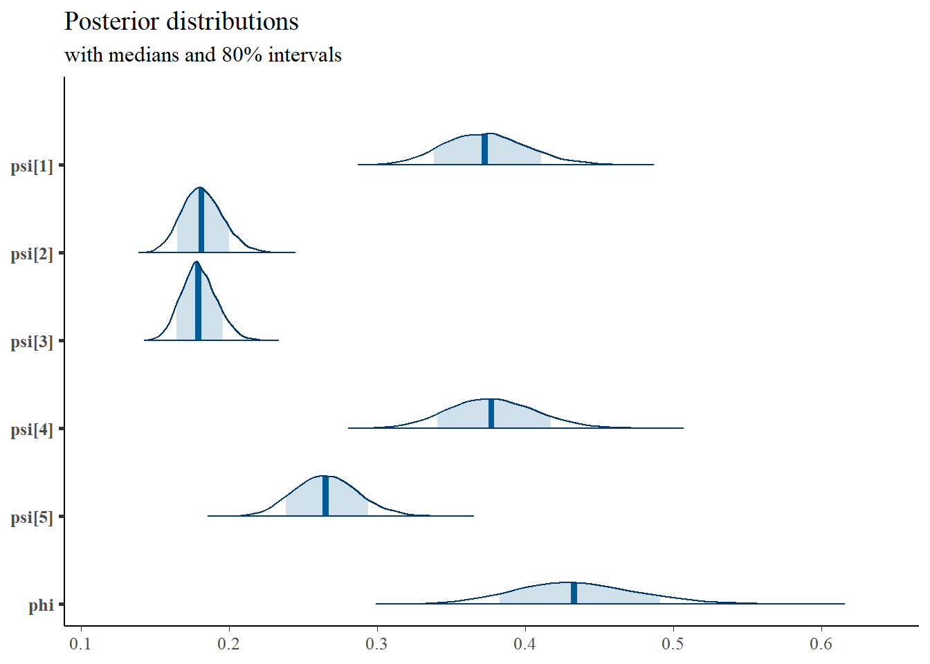
plot(fit)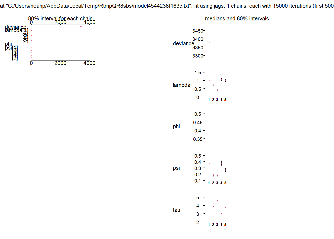
# extract posteriors for all chains
jags.mcmc <- as.mcmc(fit)


a <- colnames(as.data.frame(jags.mcmc[[1]]))
plot.data <- data.frame(as.matrix(jags.mcmc, chains=T, iters = T))
colnames(plot.data) <- c("chain", "iter", a)


plot_title <- ggtitle("Posterior distributions",
                      "with medians and 80% intervals")
mcmc_areas(
  plot.data,
  pars = c(paste0("tau[",1:5,"]")),
  prob = 0.8) +
  plot_title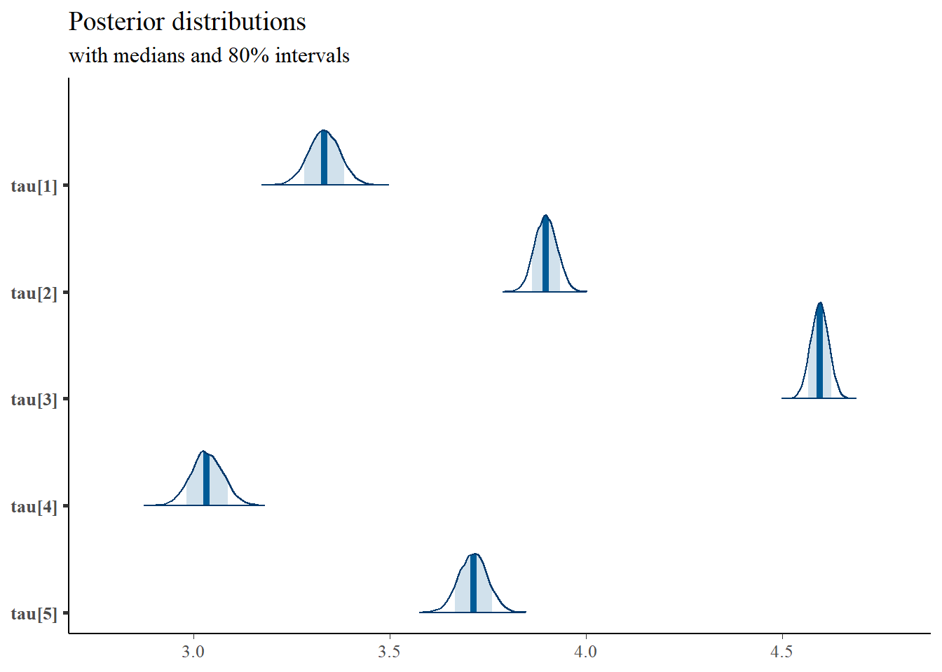
mcmc_areas(
  plot.data,
  pars = paste0("lambda[",1:5,"]"),
  prob = 0.8) +
  plot_title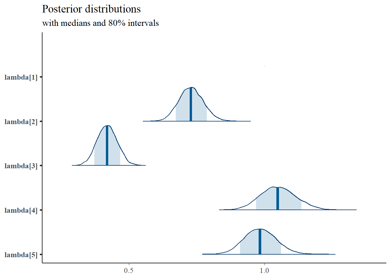
# compute model implied covariance/correlations
# for each iterations
out.mat <- matrix(ncol=10,nrow=nrow(plot.data))
colnames(out.mat) <- c("r12", "r13", "r14", "r15", "r23", "r24", "r25", "r34","r35", "r45")
plot.data1 <- cbind(plot.data,out.mat)

# compute the model implied correlations for each iterations
i <- 1
for(i in 1:nrow(plot.data1)){
  x <- plot.data1[i,]
  x <- unlist(x)
  lambda <- matrix(x[4:8], ncol=1)
  phi <- matrix(x[9], ncol=1)
  psi <- diag(x[10:14], ncol=5, nrow=5)
  micov <- lambda%*%phi%*%t(lambda)+psi
  D <- diag(sqrt(diag(micov)), ncol=5, nrow=5)
  Dinv <- solve(D)
  micor <- Dinv%*%micov%*%Dinv
  outr <- micor[lower.tri(micor)]
  # combine
  plot.data1[i,20:29] <- outr
}

obs.mat <- matrix(cor(dat)[lower.tri(cor(dat))],byrow=T,
                  ncol=10,nrow=nrow(plot.data))
colnames(obs.mat) <- c("ObsR12", "ObsR13", "ObsR14", "ObsR15", "ObsR23", "ObsR24", "ObsR25", "ObsR34","ObsR35", "ObsR45")
plot.data1 <- cbind(plot.data1,obs.mat)


theme_set(theme_classic())
t1 <- grid::textGrob('PI')
t2 <- grid::textGrob('AD')
t3 <- grid::textGrob('IGC')
t4 <- grid::textGrob('FI')
t5 <- grid::textGrob('FC')
p12 <- ggplot(plot.data1) +
  geom_density(aes(x=r12))+
  geom_vline(aes(xintercept = ObsR12), linetype="dashed")+
  lims(x=c(0.25, 0.75)) +
  labs(x=NULL,y=NULL) + theme(axis.text.y = element_blank(),axis.ticks.y = element_blank(), axis.line.y=element_blank())
p13 <- ggplot(plot.data1) +
  geom_density(aes(x=r13))+
  geom_vline(aes(xintercept = ObsR13), linetype="dashed")+
  lims(x=c(0.25, 0.75)) +
  labs(x=NULL,y=NULL) + theme(axis.text.y = element_blank(),axis.ticks.y = element_blank(), axis.line.y=element_blank())
p14 <- ggplot(plot.data1) +
  geom_density(aes(x=r14))+
  geom_vline(aes(xintercept = ObsR14), linetype="dashed")+
  lims(x=c(0.25, 0.75)) +
  labs(x=NULL,y=NULL) + theme(axis.text.y = element_blank(),axis.ticks.y = element_blank(), axis.line.y=element_blank())
p15 <- ggplot(plot.data1) +
  geom_density(aes(x=r15))+
  geom_vline(aes(xintercept = ObsR15), linetype="dashed")+
  lims(x=c(0.25, 0.75)) +
  labs(x=NULL,y=NULL) + theme(axis.text.y = element_blank(),axis.ticks.y = element_blank(), axis.line.y=element_blank())
p23 <- ggplot(plot.data1) +
  geom_density(aes(x=r23))+
  geom_vline(aes(xintercept = ObsR23), linetype="dashed")+
  lims(x=c(0.25, 0.75)) +
  labs(x=NULL,y=NULL) + theme(axis.text.y = element_blank(),axis.ticks.y = element_blank(), axis.line.y=element_blank())
p24 <- ggplot(plot.data1) +
  geom_density(aes(x=r24))+
  geom_vline(aes(xintercept = ObsR24), linetype="dashed")+
  lims(x=c(0.25, 0.75)) +
  labs(x=NULL,y=NULL) + theme(axis.text.y = element_blank(),axis.ticks.y = element_blank(), axis.line.y=element_blank())
p25 <- ggplot(plot.data1) +
  geom_density(aes(x=r25))+
  geom_vline(aes(xintercept = ObsR25), linetype="dashed")+
  lims(x=c(0.25, 0.75)) +
  labs(x=NULL,y=NULL) + theme(axis.text.y = element_blank(),axis.ticks.y = element_blank(), axis.line.y=element_blank())
p34 <- ggplot(plot.data1) +
  geom_density(aes(x=r34))+
  geom_vline(aes(xintercept = ObsR34), linetype="dashed")+
  lims(x=c(0.25, 0.75)) +
  labs(x=NULL,y=NULL) + theme(axis.text.y = element_blank(),axis.ticks.y = element_blank(), axis.line.y=element_blank())
p35 <- ggplot(plot.data1) +
  geom_density(aes(x=r35))+
  geom_vline(aes(xintercept = ObsR35), linetype="dashed")+
  lims(x=c(0.25, 0.75)) +
  labs(x=NULL,y=NULL) + theme(axis.text.y = element_blank(),axis.ticks.y = element_blank(), axis.line.y=element_blank())
p45 <- ggplot(plot.data1) +
  geom_density(aes(x=r45))+
  geom_vline(aes(xintercept = ObsR45), linetype="dashed")+
  lims(x=c(0.25, 0.75)) +
  labs(x=NULL,y=NULL) + theme(axis.text.y = element_blank(),axis.ticks.y = element_blank(), axis.line.y=element_blank())

layout <- '
A####
BC###
DEF##
GHIJ#
KLMNO
'
wrap_plots(A=t1,C=t2,F=t3,J=t4,O=t5,
           B=p12,D=p13,G=p14,K=p15,
           E=p23,H=p24,L=p25,
           I=p34,M=p35,
           N=p45,design = layout)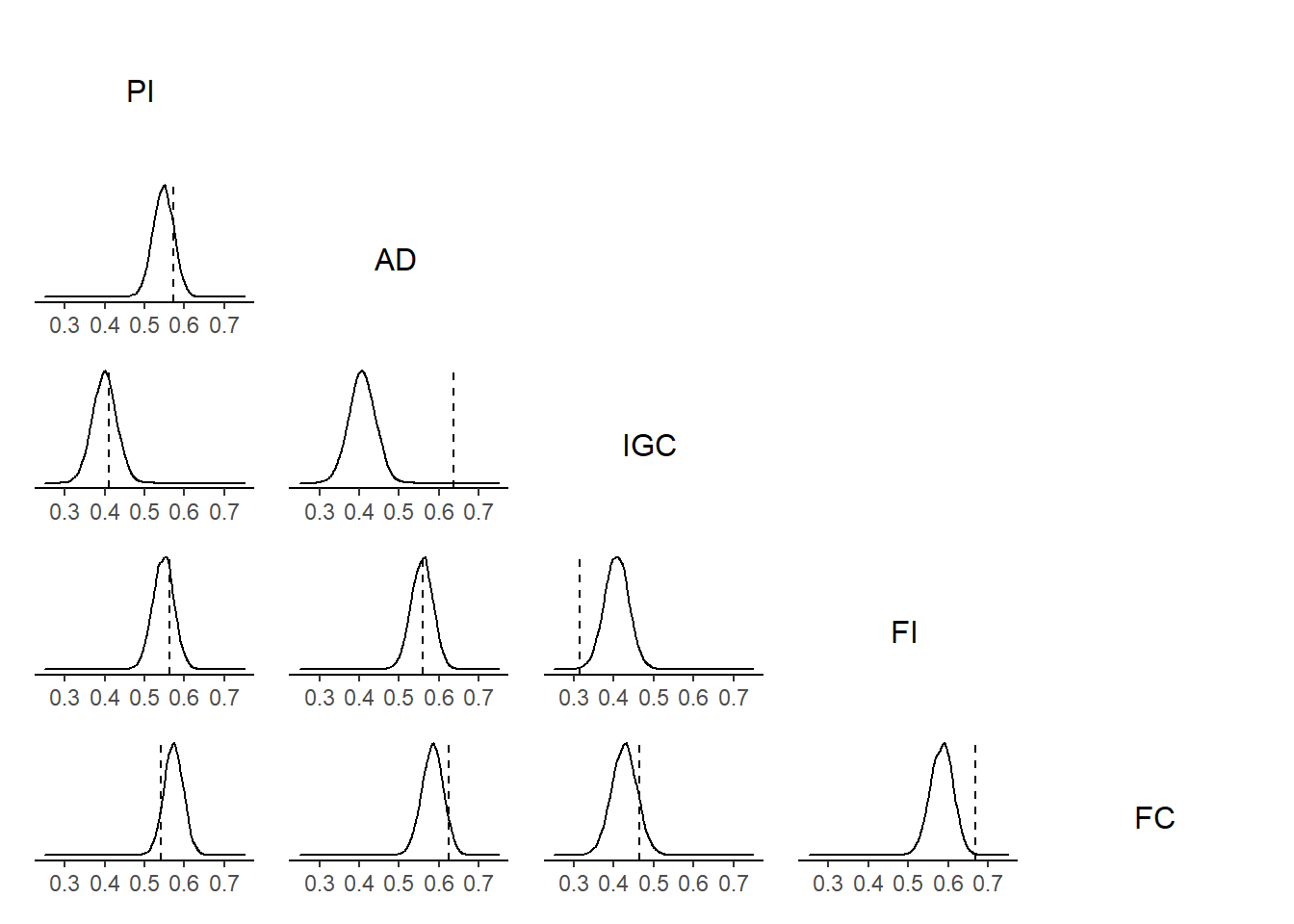
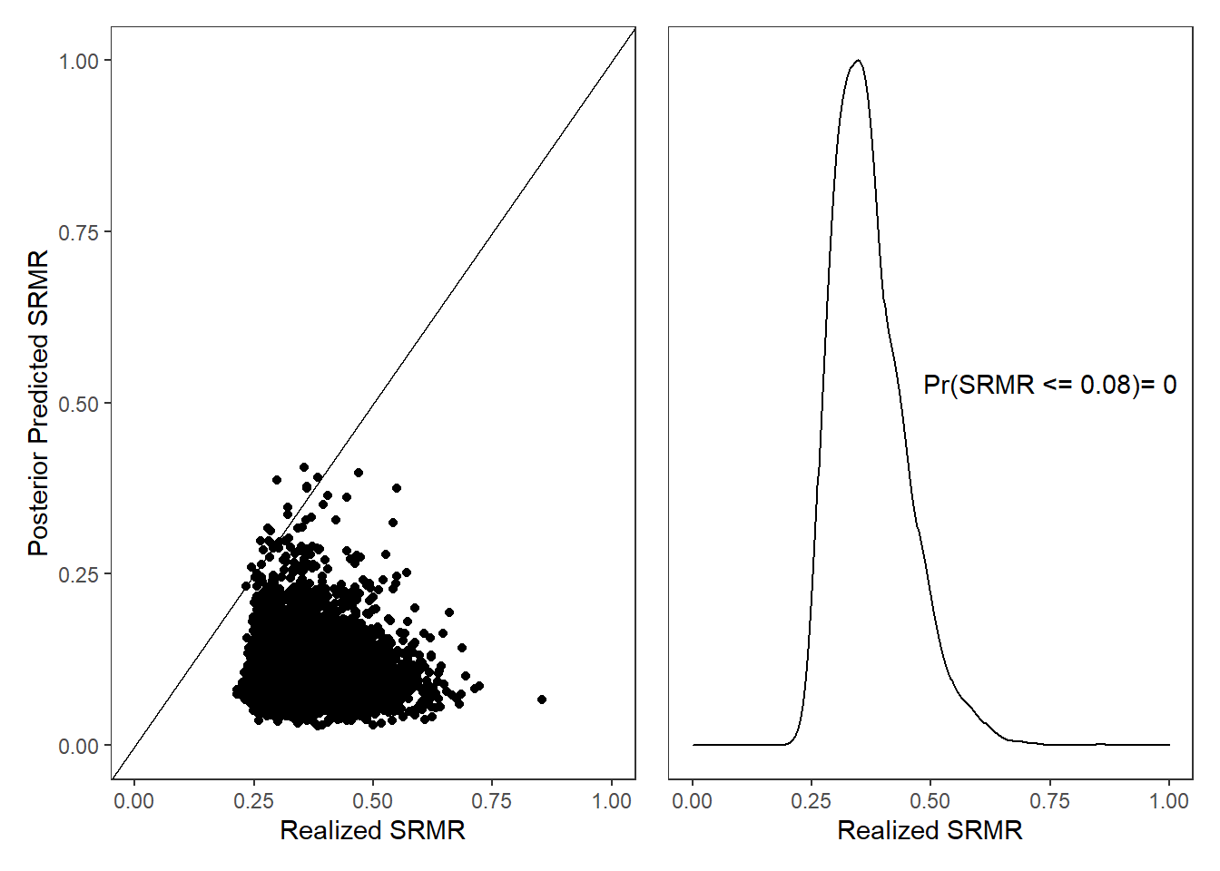
10.2.2 PPD SRMR
# model code
jags.model.cfa <- function(){

  ########################################
  # Specify the factor analysis measurement
  # model for the observables
  ########################################
  for (i in 1:n){
    for(j in 1:J){
      # model implied expectation for each observable
      mu[i,j] <- tau[j] + ksi[i]*lambda[j]
      # distribution for each observable
      x[i,j] ~ dnorm(mu[i,j], inv.psi[j])
      # Posterior Predictive Distribution of x
      #   needed for SRMR
      #   set mean to 0
      # x.ppd[i,j] ~ dnorm(0, inv.psi[j])
    }
  }

  ########################################
  # Specify the (prior) distribution for
  # the latent variables
  ########################################
  for (i in 1:n){
    # distribution for the latent variables
    ksi[i] ~ dnorm(kappa, inv.phi)
  }


  ########################################
  # Specify the prior distribution for the
  # parameters that govern the latent variables
  ########################################
  kappa <- 0              # Mean of factor 1
  inv.phi ~ dgamma(5, 10) # Precision of factor 1
  phi <- 1/inv.phi        # Variance of factor 1


  ########################################
  # Specify the prior distribution for the
  # measurement model parameters
  ########################################
  for(j in 1:J){
    tau[j] ~ dnorm(3, .1)        # Intercepts for observables
    inv.psi[j] ~ dgamma(5, 10) # Precisions for observables
    psi[j] <- 1/inv.psi[j]   # Variances for observables
  }

  lambda[1] <- 1.0              # loading fixed to 1.0
  for (j in 2:J){
    lambda[j] ~ dnorm(1, .1)    # prior distribution for the remaining loadings
  }

}
# data must be in a list
dat <- read.table("code/CFA-One-Latent-Variable/Data/IIS.dat", header=T)

mydata <- list(
  n = 500, J = 5,
  x = as.matrix(dat)
)

# vector of all parameters to save
param_save <- c("tau", paste0("lambda[",1:5,"]"), "phi", "psi")# "Sigma",

# fit model
fit <- jags(
  model.file=jags.model.cfa,
  data=mydata,
  #inits=start_values,
  parameters.to.save = param_save,
  n.iter=10000,
  n.burnin = 5000,
  n.chains = 1,
  n.thin=1,
  progress.bar = "none")
## Compiling model graph
## Resolving undeclared variables
## Allocating nodes
## Graph information:
## Observed stochastic nodes: 2500
## Unobserved stochastic nodes: 515
## Total graph size: 8029
##
## Initializing model
print(fit)## Inference for Bugs model at "C:/Users/noahp/AppData/Local/Temp/RtmpQR8sbs/model4544704352f.txt", fit using jags,
## 1 chains, each with 10000 iterations (first 5000 discarded)
## n.sims = 5000 iterations saved
## mu.vect sd.vect 2.5% 25% 50% 75% 97.5%
## lambda[1] 1.000 0.000 1.000 1.000 1.000 1.000 1.000
## lambda[2] 0.730 0.044 0.647 0.699 0.729 0.759 0.820
## lambda[3] 0.420 0.037 0.349 0.395 0.419 0.445 0.495
## lambda[4] 1.052 0.067 0.925 1.006 1.051 1.096 1.188
## lambda[5] 0.984 0.058 0.874 0.943 0.983 1.022 1.102
## phi 0.435 0.042 0.360 0.405 0.433 0.463 0.520
## psi[1] 0.373 0.028 0.322 0.354 0.372 0.392 0.432
## psi[2] 0.182 0.014 0.157 0.173 0.182 0.191 0.211
## psi[3] 0.180 0.012 0.157 0.171 0.179 0.188 0.205
## psi[4] 0.377 0.030 0.322 0.357 0.376 0.396 0.439
## psi[5] 0.266 0.022 0.225 0.251 0.266 0.281 0.311
## tau[1] 3.333 0.041 3.253 3.306 3.333 3.360 3.412
## tau[2] 3.897 0.029 3.840 3.877 3.898 3.917 3.954
## tau[3] 4.596 0.023 4.552 4.581 4.596 4.611 4.640
## tau[4] 3.033 0.042 2.952 3.005 3.034 3.062 3.115
## tau[5] 3.712 0.037 3.638 3.686 3.713 3.737 3.784
## deviance 3381.034 41.985 3299.407 3352.431 3380.812 3409.296 3463.769
##
## DIC info (using the rule, pD = var(deviance)/2)
## pD = 881.4 and DIC = 4262.4
## DIC is an estimate of expected predictive error (lower deviance is better).
# extract posteriors for all chains
jags.mcmc <- as.mcmc(fit)[[1]]

# function for estimating SRMR
SRMR.function <- function(data.cov.matrix, mod.imp.cov.matrix){

  J=nrow(data.cov.matrix)
    temp <- matrix(NA, nrow=J, ncol=J)

    for(j in 1:J){
        for(jprime in 1:j){
            temp[j, jprime] <- ((data.cov.matrix[j, jprime] - mod.imp.cov.matrix[j, jprime])/(data.cov.matrix[j, j] * data.cov.matrix[jprime, jprime]))^2
        }
    }

    SRMR <- sqrt((2*sum(temp,na.rm=TRUE))/(J*(J+1)))
    SRMR

}

# set up the parameters for
#   (1) model implied covariance
#   (2) PPD of x/covariance
iter <- nrow(jags.mcmc)
srmr.realized <- rep(NA, iter)
srmr.ppd      <- rep(NA, iter)
srmr.rpv      <- rep(NA, iter)
jags.mcmc <- cbind(jags.mcmc, srmr.realized, srmr.ppd, srmr.rpv)

N <- 500; J <- 5; M <- 1
cov.x <- cov(mydata$x)
i <- 1
for(i in 1:iter){
  # set up parameters
  x <- jags.mcmc[i,]
  lambda <- matrix(x[2:6], ncol=M, nrow=J)
  phi    <- matrix(x[7], ncol=M, nrow=M)
  psi    <- diag(x[8:12], ncol=J, nrow=J)
  # estimate model implied covariance matrix
  cov.imp <- lambda%*%phi%*%t(lambda) + psi
  # get posterior predicted observed x
  x.ppd   <- mvtnorm::rmvnorm(N, mean=rep(0, J), sigma=cov.imp)
  # compute posterior predictied covariance matrix
  cov.ppd <- cov(x.ppd)
  # estimate SRMR values
  jags.mcmc[i,18] <- SRMR.function(cov.x, cov.imp)# srmr realized
  jags.mcmc[i,19] <- SRMR.function(cov.ppd, cov.imp)# srmr ppd
  # posterior predicted p-value of realized SRMR being <= 0.08.
  jags.mcmc[i,20] <- ifelse(jags.mcmc[i,18]<=0.08, 1, 0)
}

plot.dat <- as.data.frame(jags.mcmc)

p1 <- ggplot(plot.dat, aes(x=srmr.realized, y=srmr.ppd))+
  geom_point()+
  geom_abline(slope=1, intercept = 0)+
  lims(x=c(0,1),y=c(0,1))+
  labs(x="Realized SRMR",y="Posterior Predicted SRMR") +
  theme_bw()+theme(panel.grid = element_blank())
p2 <- ggplot(plot.dat, aes(x=srmr.realized))+
  geom_density()+
  lims(x=c(0,1))+
  labs(x="Realized SRMR", y=NULL) +
  annotate("text", x = 0.75, y = 3,
           label = paste0("Pr(SRMR <= 0.08)= ",
                          round(mean(plot.dat$srmr.rpv), 2))) +
  theme_bw()+theme(panel.grid = element_blank(),
                   axis.text.y = element_blank(),
                   axis.ticks.y = element_blank())
p1 + p2