13 Latent Class Analysis
Latent class analysis (LCA) takes a different approach to modeling latent variables than has been discussed in the previous chapters (especially CFA or IRT). The major distinguishing aspect of LCA is that the latent variable is hypothesized to be a discrete random variable as opposed to a continuous random variable. This shift in perspective is beneficial to researchers/analysts wishing to think categorically and discuss groups of observations/people/units as opposed to a dimension of possible differences.
LCA is often used in an exploratory nature to try to identify the number of “latent classes” or unobserved groups. However, in the text, Levy and Mislevy discuss what they describe as a more “confirmatory” approach to LCA. The major distinction is that they specify the number of classes to be known, and treat this chapter as a resource for how to estimate the model within a Bayesian framework.
To extend their work, we have added a section on model selection and provided resources for the interested reader. But, in general, the topic of model selection in Bayesian LCA (and Bayesian SEM more generally) is still an ongoing area of research. Many views exist on how to conduct model selection (if at all) and we will try to present an array of options that have been proposed.
13.1 LCA Model Specification
LCA is a finite mixture model. A mixture model is generally any statistical model that combines distributions to describe different subsets or aspects of the data. For example, LCA is a mixture model that posits class specific item/indicator response probabilities. Different classes have a different distribution or expected response on average. Each unit of observation (e.g., person) is assumed to belong to 1 and only 1 class. Because individuals can only belong to one class, the different classes of observations make up different subsets of the data used in the analysis. One result of an LCA model is the ability to identify the likelihood that an individual belongs to a particular class which is sometimes called probabilistic clustering.
Let \(x_{ij}\) be the observed value from respondent \(i=1, \ldots, N\) on observable (item) \(j=1, \ldots, J\). Because \(x\) is binary, the observed value can be \(0\) or \(1\). The latent class variable commonly denoted with a \(C\) to represent the total number of latent classes. Let \(\theta_i\) represent the class for individual \(i\), where \(\theta_i \in \lbrace 1, \ldots, C\rbrace\). Similar to IRT, LCA models the probability of the observed response. However, LCA we estimate this value more directly because the value only depends on latent class membership instead of the value being indirectly estimated through item difficulties and discrimination parameters. The model for the observed response being 1 is \[p(x_{ij} = 1) = \sum_{c=1}^Cp(x_{ij}=1\mid\theta_i=c,\pi_j)\gamma_c,\] where,
- \(p(x_{ij}=1\mid\theta_i=c,\pi_i)\) is class specific conditional response probability to item \(i\),
- \(\pi_j\) represents the item parameters, in this case it is simply the conditional probability, but can be expanded to be a set of item parameters (e.g., IRT-like),
- \(\gamma_c\) represents the class mixing weight or the class size parameter. The size of each class helps to identify how likely an individual in to be in any of the \(C\) classes if we had no other information.
- Additionally, the class mixing weights always sums to \(1\), that is
\[\sum_{c=1}^C\gamma_c = \sum_{c=1}^Cp(\theta_i=c) = 1.\]
Another way of interpreting the mixing weight is as a class proportion. This framing can sometimes make it easier to see that the indicator response probability is a weighted average of response probabilities over the \(C\) classes. The larger the class the more that class influences the expected response probabilities.
13.1.1 LCA Model Indeterminacy
One common aspect of LCA than can be a bit of a headache at times if not carefully considered is an issue known as label switching. LCA models discrete latent variables which do not have any inherent labels, as CFA/IRT model continuous latent variables that do not have any inherent scale/metric.
13.1.2 Model Likelihood
The likelihood function for LCA follows a similar development as the likelihood function from CFA and IRT. We assume that the individuals are independent (\(i\)’s are exchangeable). We assume that the responses to each item are conditionally (locally) independent (\(j\)’s are exchangeable). The joint probability conditional on the latent variable \(C\) is
\[p(\mathbf{x}_i \vert \boldsymbol{\theta}, \boldsymbol{\pi}) = \prod_{i=1}^Np(\mathbf{x}_i \vert \theta_i=c, \boldsymbol{\pi}) = \prod_{i=1}^N\prod_{j=1}^Jp(x_{ij} \vert \theta_i=c, \pi_j).\]
The marginal probability when the observed data when we sum over the possible latent classes becomes
\[\begin{align*} p(\mathbf{x}_i \vert \boldsymbol{\pi}, \boldsymbol{\gamma}) &= \prod_{i=1}^N\sum_{c=1}^C p(\mathbf{x}_i \vert \theta_i=c, \boldsymbol{\pi})p(\theta_i = c \vert \gamma)\\ &= \prod_{i=1}^N\left(\sum_{c=1}^C \left(\prod_{j=1}^J p(x_{ij} \vert \theta_i=c, \pi_j)\right)p(\theta_i = c \vert \gamma)\right) \end{align*} \]
13.2 Bayesian LCA Model Specification
For the Bayesian formulation of the LCA model, the construction will be carried out in pieces similar to previous chapters.
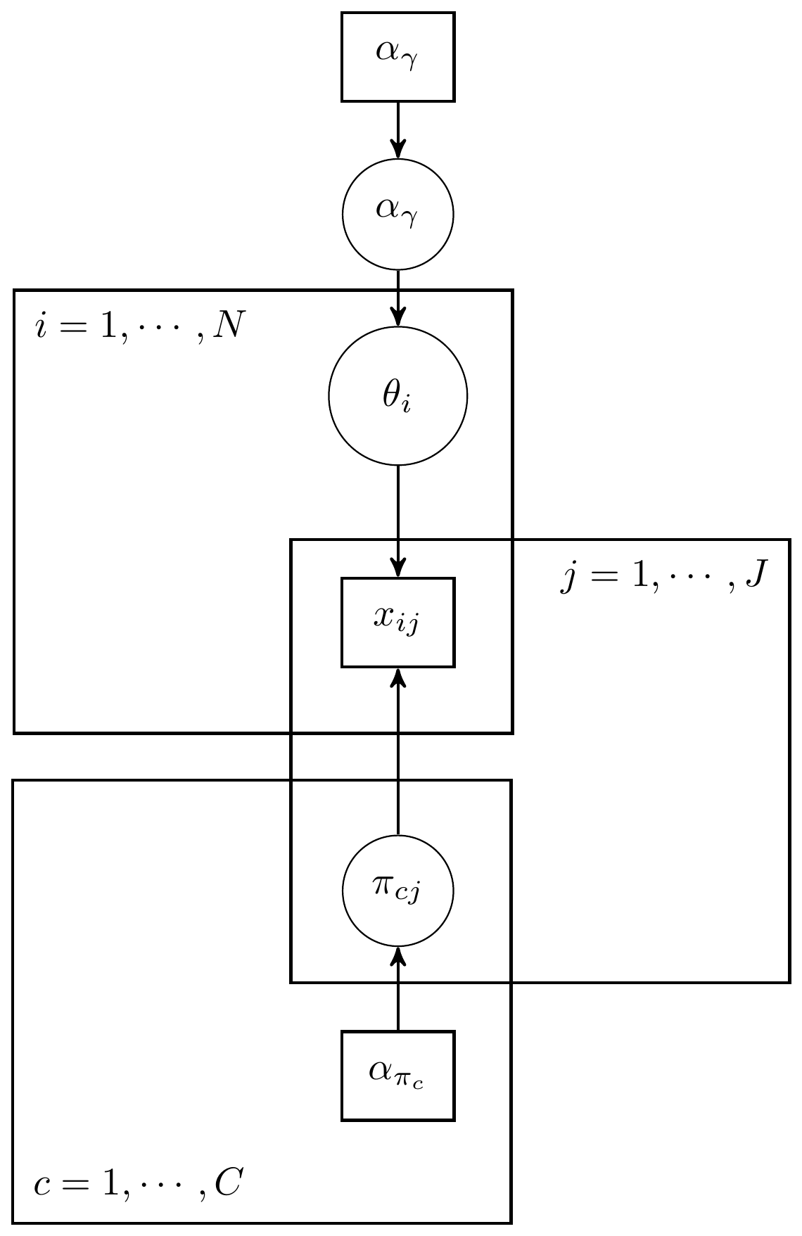
Figure 13.1: DAG for a general latent class analysis model
13.2.1 Distribution of Observed Indicators
First, the distribution of the observed variables is specified as a product of independent probabilities. That is, the observed data distribution is categorical(.). Or
\[\begin{align*} p(\mathbf{x}\vert \boldsymbol{\theta}, \boldsymbol{\pi})&= \prod_{i=1}^N p(\mathbf{x}_i\vert \theta_i, \boldsymbol{\pi}) = \prod_{i=1}^N \prod_{j=1}^J p(x_{ij}\vert \theta_i, \boldsymbol{\pi}_j),\\ x_{ij} &\sim \mathrm{Categorical}(\pi_{cj})\\ \end{align*}\] where the model holds for observables taking values coded as \(1,...,K\) with the categorical indicators. One of the major changes from an IRT model is that the latent variables are categorical, resulting in a different distribution for the latent variable. The Dirichlet distribution is commonly used as the prior for the categorical latent variables. The Dirichlet distribution is a generalization of the Beta distribution to more than two district outcomes. The distribution models the categorical data as the likelihood or propensity to be one of the categoricals.
13.2.2 Prior Distributions
The LCA model, as described here, contains two major types of parameters. That is, (1) the latent class status for each respondent and (2) the class specific category proportions. These two parameter types are vectors over respondents and items, respectively. The joint prior distribution can be generally described as \[p(\theta, \pi) = p(\theta)p(\pi),\] due to assuming independence between these two types of parameters. Independence is a logical assumption and aligns with the IRT and CFA traditions that latent variable values are independent of the measurement model parameters.
The prior for the latent variables is represents the prior for the discrete groups respondents are assumed to belong to. A common prior is placed over all respondents \[p(\theta)=\prod_{i=1}^np(\theta_i\vert\boldsymbol{\theta}_p),\] where \(\boldsymbol\theta_p\) represents the hyperpriors defining the conditions of the categorical latent variables. The vector of parameters \(\boldsymbol\theta_p = \boldsymbol\gamma = (\gamma_1, \gamma_2, ..., \gamma_C)\), where \(C\) is the number of latent groups. Stated in another way, \[\theta_i | \boldsymbol\gamma \sim \mathrm{Categorical}(\boldsymbol\gamma).\]
The hyperprior for the categorical latent variable is also commonly given a prior distribution. The \(\boldsymbol\gamma\) parameters represent the class proportions and a prior on these parameters is useful when these class proportions are not known. The prior is \[\boldsymbol\gamma \sim \mathrm{Dirichlet}(\boldsymbol\alpha_\gamma),\] where \(\boldsymbol\alpha_\gamma = (\alpha_{\gamma 1}, \alpha_{\gamma 2}, ..., \alpha_{\gamma C}).\) The Dirichlet distribution is a generalization of the Beta distribution to more than two categories. This allows for a useful representation of the probabilities with well known statistical and sampling properties.
The priors for the measurement model parameters (\(\boldsymbol\pi\)) are commonly defined at the item level instead of jointly over all items: \[p(\boldsymbol\pi) = \prod_{j=1}^Jp(\boldsymbol\pi_j\vert\boldsymbol\alpha_\pi),\] where \(\boldsymbol\alpha_\pi\) defines the hyperpriors for the measurement model parameters. The measurement model commonly utilizes either dichotomous or categorical indicators which leads to the use of either the Beta distribution or Dirichlet distribution for the priors.
13.2.3 Full Model Specification
The full model specification can be shown as follows:
\[ \begin{align*} p(\boldsymbol\theta, \boldsymbol\gamma, \boldsymbol\pi) &\propto p(\mathbf{x} \vert \boldsymbol\theta, \boldsymbol\gamma, \boldsymbol\pi) p(\boldsymbol\theta, \boldsymbol\gamma, \boldsymbol\pi)\\ &= p(\mathbf{x} \vert \boldsymbol\theta, \boldsymbol\gamma, \boldsymbol\pi) p(\boldsymbol\theta) p(\boldsymbol\gamma) p(\boldsymbol\pi)\\ &= \prod_{i=1}^N \prod_{j=1}^J p(x_{ij}\vert \theta_i, \boldsymbol{\pi}_j)p(\theta_i \vert \boldsymbol\gamma)p(\boldsymbol\gamma) \prod_{c=1}^Cp(\boldsymbol\pi_{cj})\\ (x_{ij} \vert \theta_i=c, \boldsymbol{\pi}_j) &\sim \mathrm{Categorical}(\boldsymbol{\pi}_{cj}), \mathrm{for}\ i=1, ...,n,\ j=1, ...,J,\\ \theta_i \vert \boldsymbol{\gamma} &\sim \mathrm{Categorical}(\boldsymbol{\gamma})\ \mathrm{for}\ i=1, ...,n,\\ \boldsymbol\gamma &\sim \mathrm{Dirichlet}(\boldsymbol\alpha_{\gamma}),\\ \boldsymbol\pi_{cj} &\sim \mathrm{Dirichlet}(\boldsymbol\alpha_{\pi_c})\ \mathrm{for}\ c=1, ..., C, j=1, ..., J. \end{align*} \]
13.3 Academic Cheating Example
The academic cheating example is discussed on pages 328-340. The last few pages pertain mainly to model fit/evaluation and a discussion on indeterminacy in the model. Some of these points will be left to the reader for in-text learning. The major motivation for this current development is applying the model from pages 329-330, and replicating results (p.336).
13.3.1 Estimating using JAGS
jags.model.lsat <- function(){

#########################################
# Specify the item response measurement model for the observables
#########################################
for (i in 1:n){
  for(j in 1:J){
    x[i,j] ~ dbern(pi[theta[i],j])                  # distribution for each observable conditional on latent class assignment theta
  }
}


##########################################
# Specify the (prior) distribution for the latent variables
##########################################
for (i in 1:n){
  theta[i] ~ dcat(gamma[])  # distribution for the latent variables is categorical
}

gamma[1:C] ~ ddirich(alpha_gamma[])
for(c in 1:C){
  alpha_gamma[c] = 1
}

##########################################
# Specify the prior distribution for the measurement model parameters
# Measurement model consists of class specific response probabilities
##########################################
for(c in 1:C){
  for(j in 1:(J-1)){
    pi[c,j] ~ dbeta(1,1)
  }
}
pi[1,J] ~ dbeta(1,1)
pi[2,J] ~ dbeta(1,1)


} # closes the model

# initial values
start_values <- list(
  list("gamma"=c(0.9, 0.1),
       "pi"=structure(.Data=c(.37, .20, .06, .04, .41, .47, .19, .32), .Dim=c(2, 4))),
  list("gamma"=c(0.1, 0.9),
       "pi"=structure(.Data=c(.58, .62, .69, .77, .81, .84, .88, .90), .Dim=c(2, 4))),
  list("gamma"=c(0.5, 0.5),
       "pi"=structure(.Data=c(.32, .49, .29, .61, .48, .54, .44, .70), .Dim=c(2, 4)))
)

# vector of all parameters to save
param_save <- c("gamma", "pi")

# dataset
dat <- read.table("data/Cheat.dat", header=F)

mydata <- list(
  n = nrow(dat),
  J = ncol(dat),
  C=2,
  x = as.matrix(dat)
)

# fit model
fit <- jags(
  model.file=jags.model.lsat,
  data=mydata,
  inits=start_values,
  parameters.to.save = param_save,
  n.iter=2000,
  n.burnin = 1000,
  n.chains = 3,
  progress.bar = "none")
## module glm loaded## Compiling model graph
## Resolving undeclared variables
## Allocating nodes
## Graph information:
## Observed stochastic nodes: 1276
## Unobserved stochastic nodes: 328
## Total graph size: 2885
##
## Initializing model
print(fit)## Inference for Bugs model at "C:/Users/noahp/AppData/Local/Temp/Rtmp4WWggD/model5c285c9023ab.txt", fit using jags,
## 3 chains, each with 2000 iterations (first 1000 discarded)
## n.sims = 3000 iterations saved
## mu.vect sd.vect 2.5% 25% 50% 75% 97.5% Rhat n.eff
## gamma[1] 0.861 0.063 0.757 0.839 0.870 0.895 0.937 1.239 73
## gamma[2] 0.139 0.063 0.063 0.105 0.130 0.161 0.243 1.041 77
## pi[1,1] 0.033 0.018 0.003 0.020 0.032 0.044 0.073 1.058 80
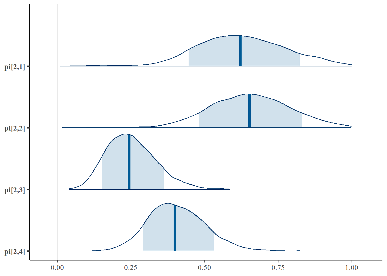
## pi[2,1] 0.626 0.147 0.359 0.526 0.622 0.728 0.913 1.028 180
## pi[1,2] 0.042 0.021 0.004 0.026 0.041 0.056 0.086 1.005 610
## pi[2,2] 0.652 0.139 0.382 0.560 0.653 0.746 0.919 1.050 92
## pi[1,3] 0.043 0.015 0.016 0.033 0.042 0.052 0.074 1.026 640
## pi[2,3] 0.252 0.084 0.112 0.190 0.244 0.305 0.439 1.011 190
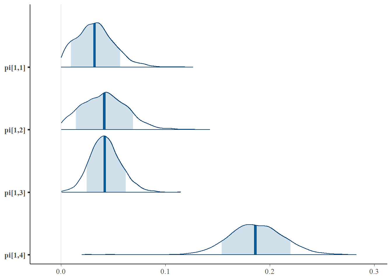
## pi[1,4] 0.186 0.027 0.136 0.170 0.186 0.204 0.238 1.065 230
## pi[2,4] 0.406 0.096 0.233 0.338 0.399 0.469 0.608 1.002 1100
## deviance 735.481 29.161 681.307 718.188 734.787 751.019 789.102 1.004 3000
##
## For each parameter, n.eff is a crude measure of effective sample size,
## and Rhat is the potential scale reduction factor (at convergence, Rhat=1).
##
## DIC info (using the rule, pD = var(deviance)/2)
## pD = 425.4 and DIC = 1160.9
## DIC is an estimate of expected predictive error (lower deviance is better).
# extract posteriors for all chains
jags.mcmc <- as.mcmc(fit)
# the below two plots are too big to be useful given the 1000 observations.
#R2jags::traceplot(jags.mcmc)

# gelman-rubin-brook
#gelman.plot(jags.mcmc)

# convert to single data.frame for density plot
a <- colnames(as.data.frame(jags.mcmc[[1]]))
plot.data <- data.frame(as.matrix(jags.mcmc, chains=T, iters = T))
colnames(plot.data) <- c("chain", "iter", a)


bayesplot::mcmc_acf(plot.data,pars = c(paste0("gamma[", 1:2, "]")))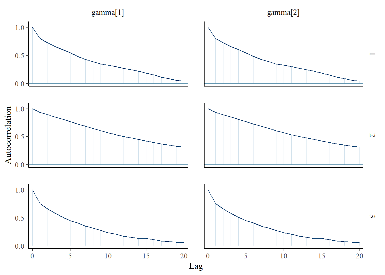
bayesplot::mcmc_trace(plot.data,pars = c(paste0("gamma[", 1:2, "]")))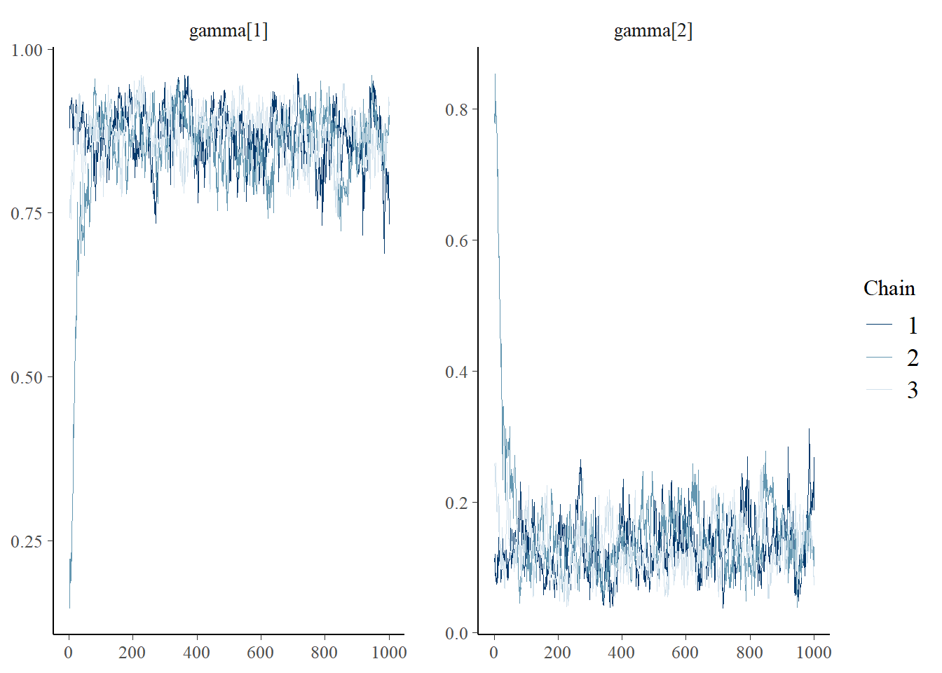
ggmcmc::ggs_grb(ggs(jags.mcmc), family="gamma")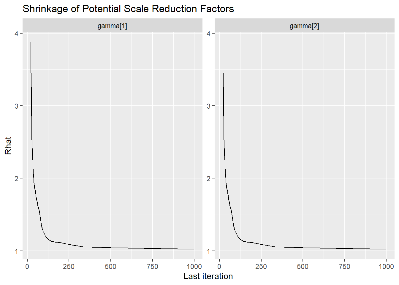
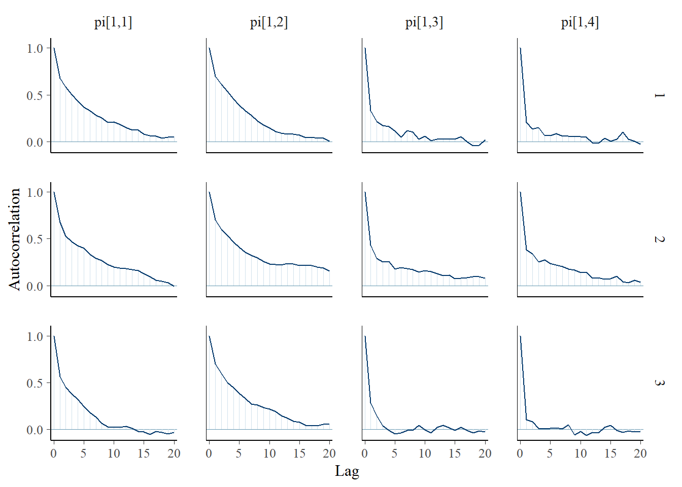
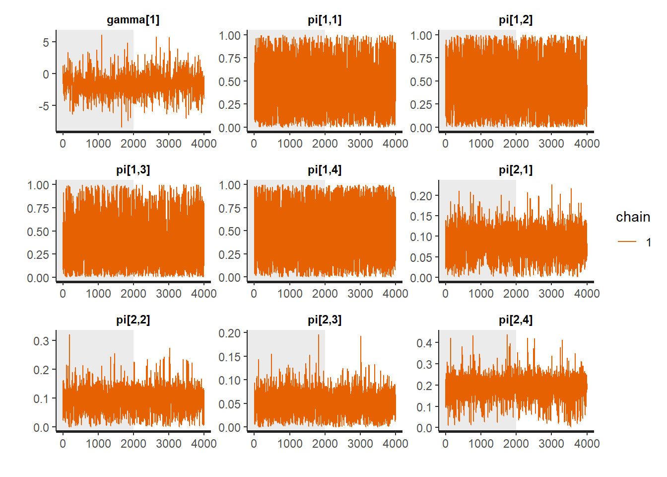
bayesplot::mcmc_trace(plot.data,pars = c(paste0("pi[1,", 1:4, "]")))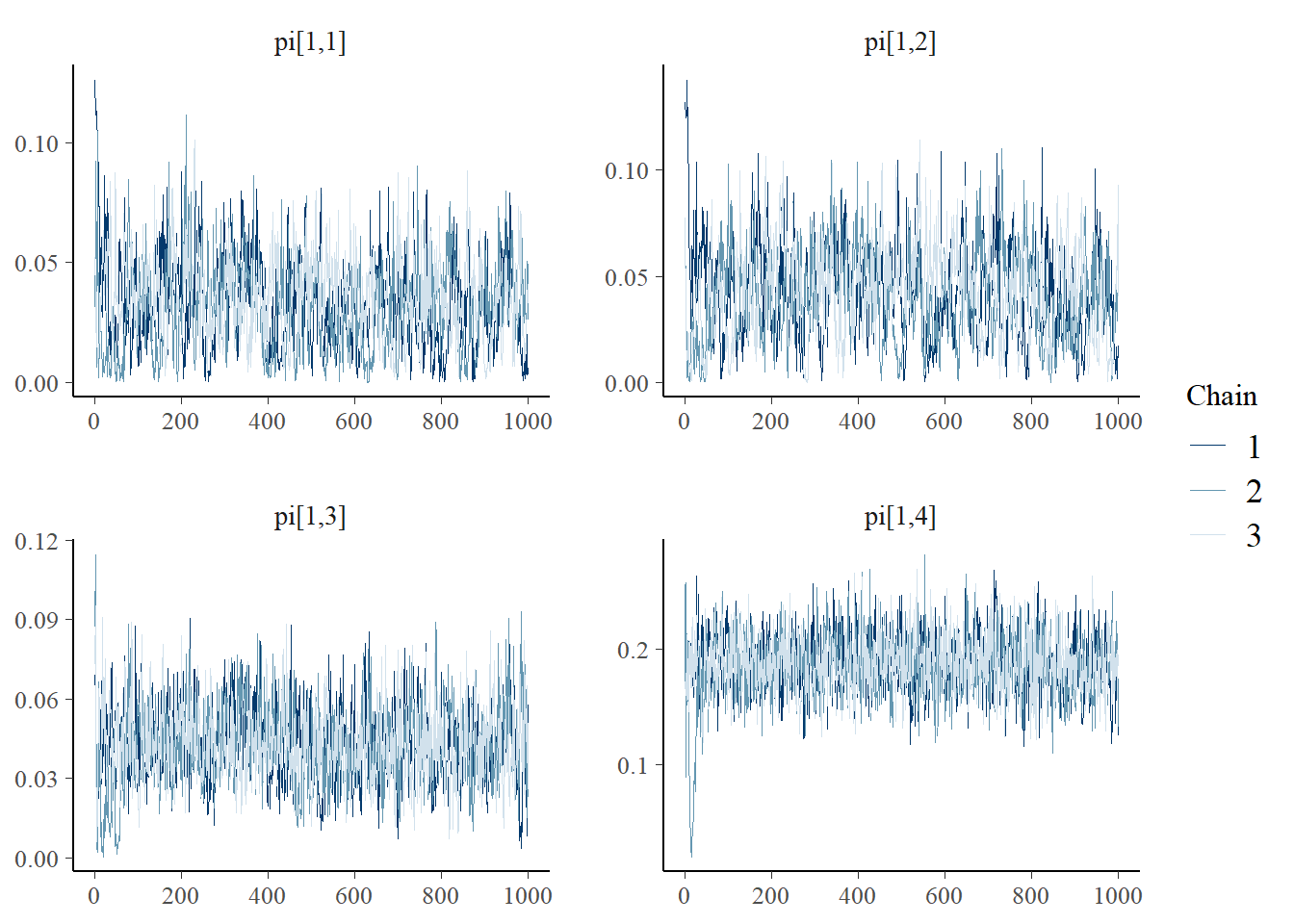
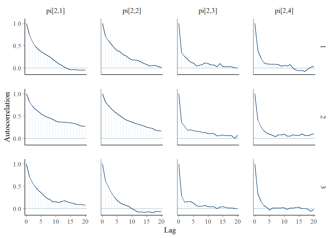
bayesplot::mcmc_trace(plot.data,pars = c(paste0("pi[2,", 1:4, "]")))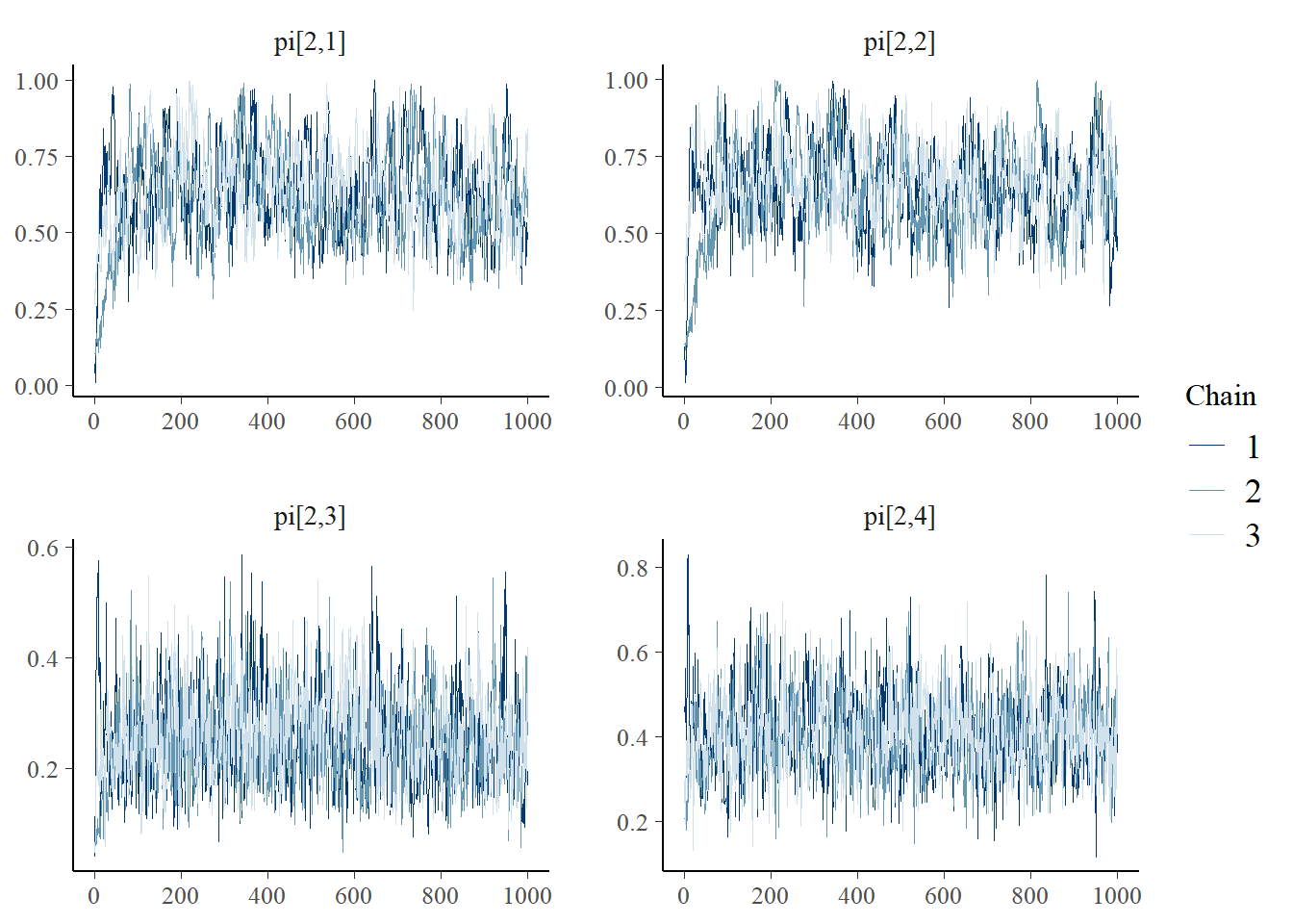
ggmcmc::ggs_grb(ggs(jags.mcmc), family="pi")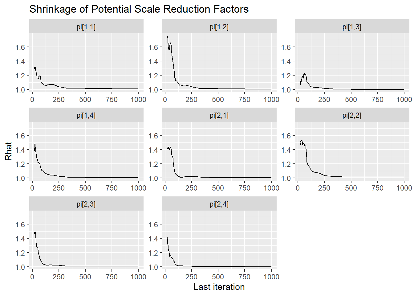
13.3.2 Estimation using Stan
model_lca <- [1717 chars quoted with ''']


# initial values
start_values <- list(
  list(gamma=c(0.1, 0.9),
       pi=structure(.Data=c(.37, .20, .06, .04, .41, .47, .19, .32), .Dim=c(2, 4))),
  list(gamma=c(0.2, 0.8),
       pi=structure(.Data=c(.58, .62, .69, .77, .81, .84, .88, .90), .Dim=c(2, 4))),
  list(gamma=c(0.4, 0.6),
       pi=structure(.Data=c(.32, .49, .29, .61, .48, .54, .44, .70), .Dim=c(2, 4)))
)

# dataset
dat <- read.table("data/Cheat.dat", header=F)

mydata <- list(
  N = nrow(dat),
  J = ncol(dat),
  C = 2,
  x = as.matrix(dat)
)


# Next, need to fit the model
#   I have explicitly outlined some common parameters
fit <- stan(
  model_code = model_lca, # model code to be compiled
  data = mydata,          # my data
  #init = start_values,    # starting values
  chains = 1,             # number of Markov chains
  warmup = 2000,          # number of warm up iterations per chain
  iter = 4000,            # total number of iterations per chain
  cores = 1,              # number of cores (could use one per chain)
  #refresh = 0             # no progress shown
)
##
## SAMPLING FOR MODEL 'anon_model' NOW (CHAIN 1).
## Chain 1:
## Chain 1: Gradient evaluation took 0.000971 seconds
## Chain 1: 1000 transitions using 10 leapfrog steps per transition would take 9.71 seconds.
## Chain 1: Adjust your expectations accordingly!
## Chain 1:
## Chain 1:
## Chain 1: Iteration: 1 / 4000 [ 0%] (Warmup)
## Chain 1: Iteration: 400 / 4000 [ 10%] (Warmup)
## Chain 1: Iteration: 800 / 4000 [ 20%] (Warmup)
## Chain 1: Iteration: 1200 / 4000 [ 30%] (Warmup)
## Chain 1: Iteration: 1600 / 4000 [ 40%] (Warmup)
## Chain 1: Iteration: 2000 / 4000 [ 50%] (Warmup)
## Chain 1: Iteration: 2001 / 4000 [ 50%] (Sampling)
## Chain 1: Iteration: 2400 / 4000 [ 60%] (Sampling)
## Chain 1: Iteration: 2800 / 4000 [ 70%] (Sampling)
## Chain 1: Iteration: 3200 / 4000 [ 80%] (Sampling)
## Chain 1: Iteration: 3600 / 4000 [ 90%] (Sampling)
## Chain 1: Iteration: 4000 / 4000 [100%] (Sampling)
## Chain 1:
## Chain 1: Elapsed Time: 34.55 seconds (Warm-up)
## Chain 1: 30.385 seconds (Sampling)
## Chain 1: 64.935 seconds (Total)
## Chain 1:## Inference for Stan model: anon_model.
## 1 chains, each with iter=4000; warmup=2000; thin=1;
## post-warmup draws per chain=2000, total post-warmup draws=2000.
##
## mean se_mean sd 2.5% 25% 50% 75% 97.5% n_eff Rhat
## gamma[1] -1.50 0.06 1.43 -4.48 -2.26 -1.50 -0.79 1.60 549 1
## gamma_ord[1] 0.12 0.00 0.10 0.01 0.05 0.09 0.16 0.42 548 1
## gamma_ord[2] 0.88 0.00 0.10 0.58 0.84 0.91 0.95 0.99 548 1
## pi[1,1] 0.43 0.01 0.28 0.02 0.19 0.38 0.64 0.96 893 1
## pi[1,2] 0.44 0.01 0.28 0.01 0.18 0.41 0.67 0.96 922 1
## pi[1,3] 0.36 0.01 0.26 0.02 0.14 0.31 0.55 0.93 874 1
## pi[1,4] 0.48 0.01 0.29 0.03 0.23 0.46 0.73 0.97 1193 1
## pi[2,1] 0.08 0.00 0.04 0.01 0.05 0.08 0.11 0.15 777 1
## pi[2,2] 0.09 0.00 0.04 0.01 0.07 0.10 0.12 0.17 817 1
## pi[2,3] 0.05 0.00 0.03 0.00 0.03 0.05 0.06 0.10 631 1
## pi[2,4] 0.18 0.00 0.06 0.04 0.15 0.19 0.22 0.28 532 1
##
## Samples were drawn using NUTS(diag_e) at Sun Jul 17 14:53:30 2022.
## For each parameter, n_eff is a crude measure of effective sample size,
## and Rhat is the potential scale reduction factor on split chains (at
## convergence, Rhat=1).
# plot the posterior in a
#  95% probability interval
#  and 80% to contrast the dispersion
plot(fit,pars =c("gamma", "pi"))
## ci_level: 0.8 (80% intervals)## outer_level: 0.95 (95% intervals)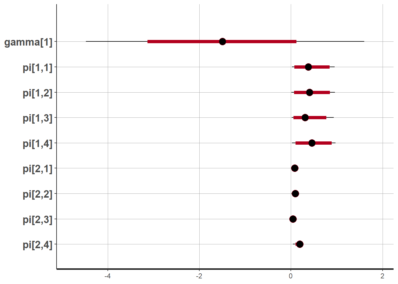
# Gelman-Rubin-Brooks Convergence Criterion
ggs_grb(ggs(fit, family = c("gamma"))) +
   theme_bw() + theme(panel.grid = element_blank())
## Error in ggs_grb(ggs(fit, family = c("gamma"))): At least two chains are required
ggs_grb(ggs(fit, family = "pi")) +
   theme_bw() + theme(panel.grid = element_blank())
## Error in ggs_grb(ggs(fit, family = "pi")): At least two chains are required
# autocorrelation
ggs_autocorrelation(ggs(fit, family="gamma")) +
   theme_bw() + theme(panel.grid = element_blank())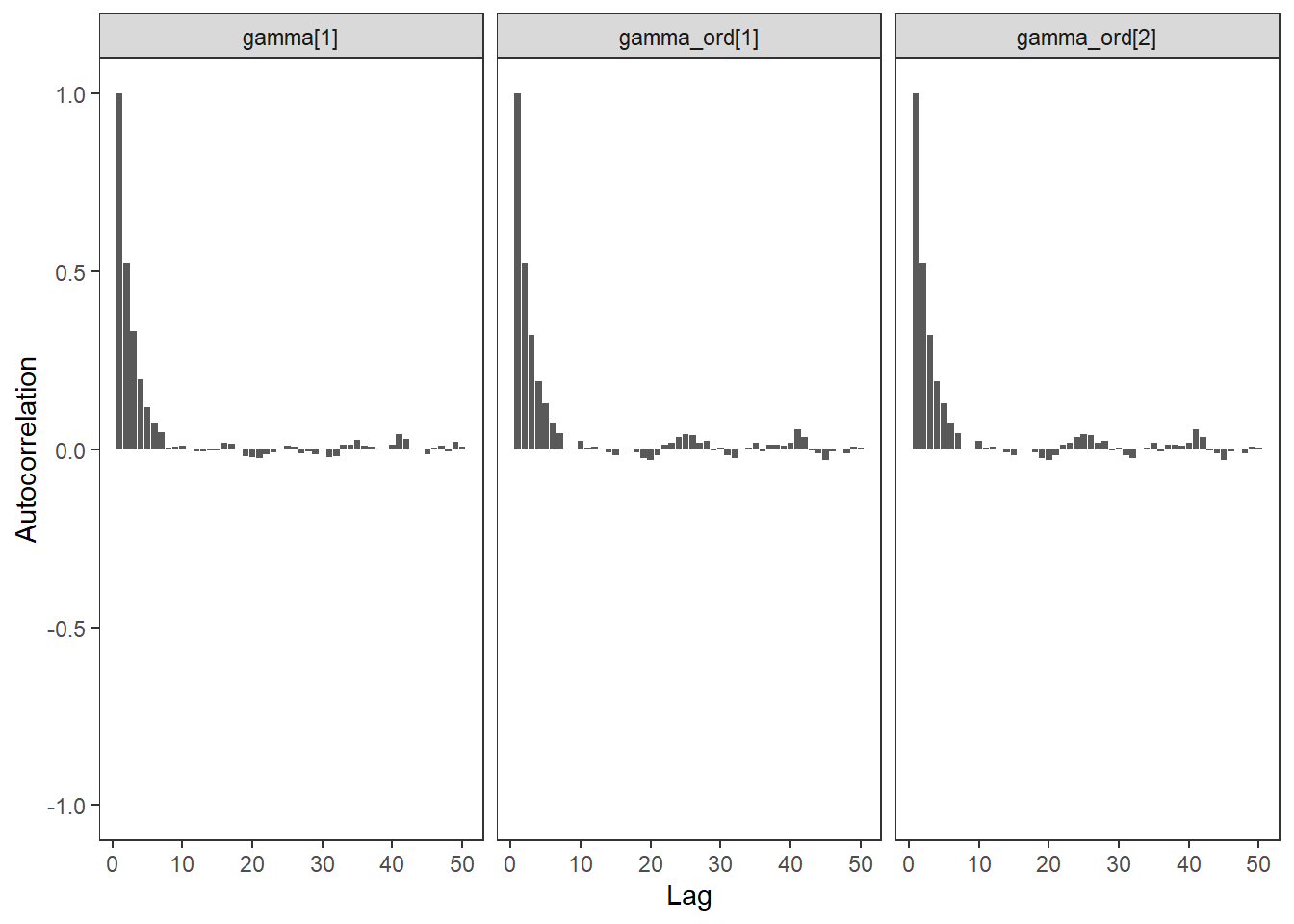
ggs_autocorrelation(ggs(fit, family="pi")) +
   theme_bw() + theme(panel.grid = element_blank())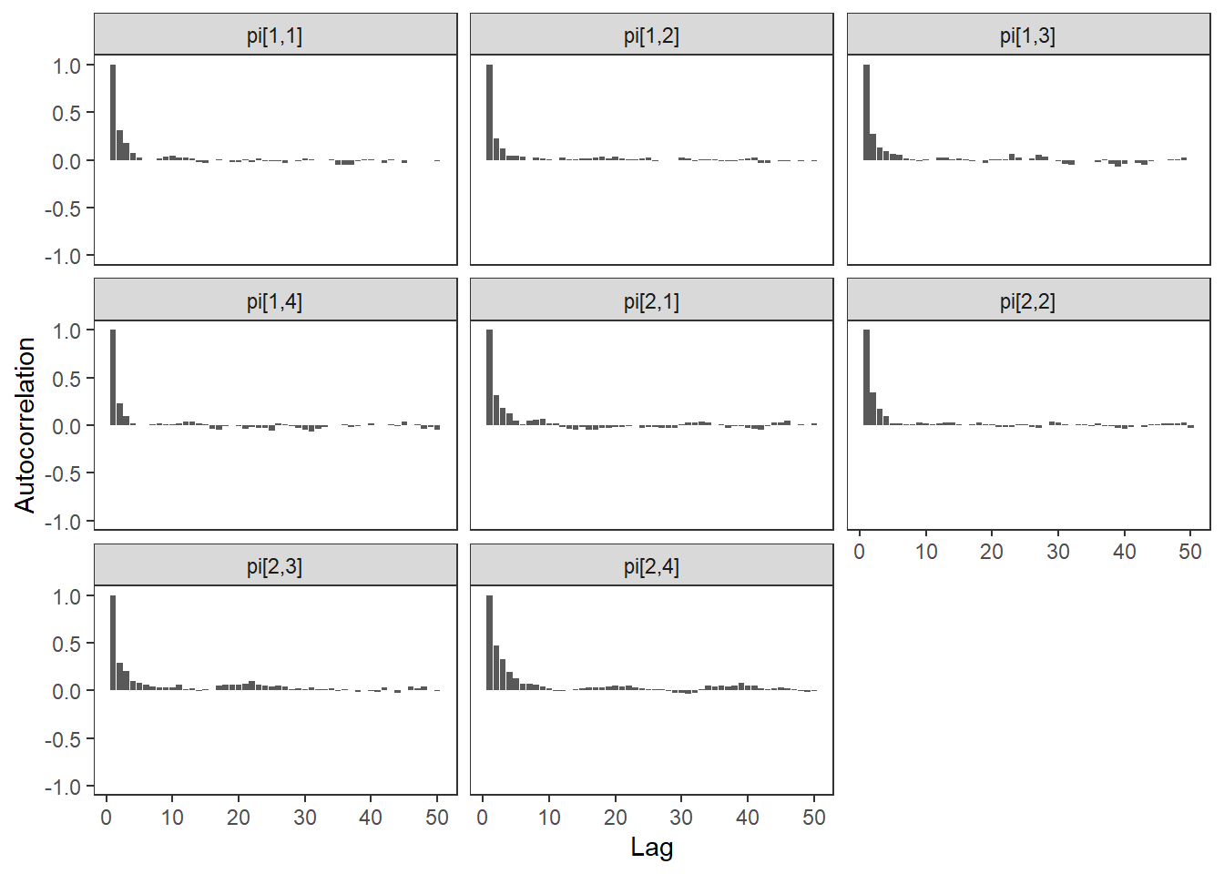
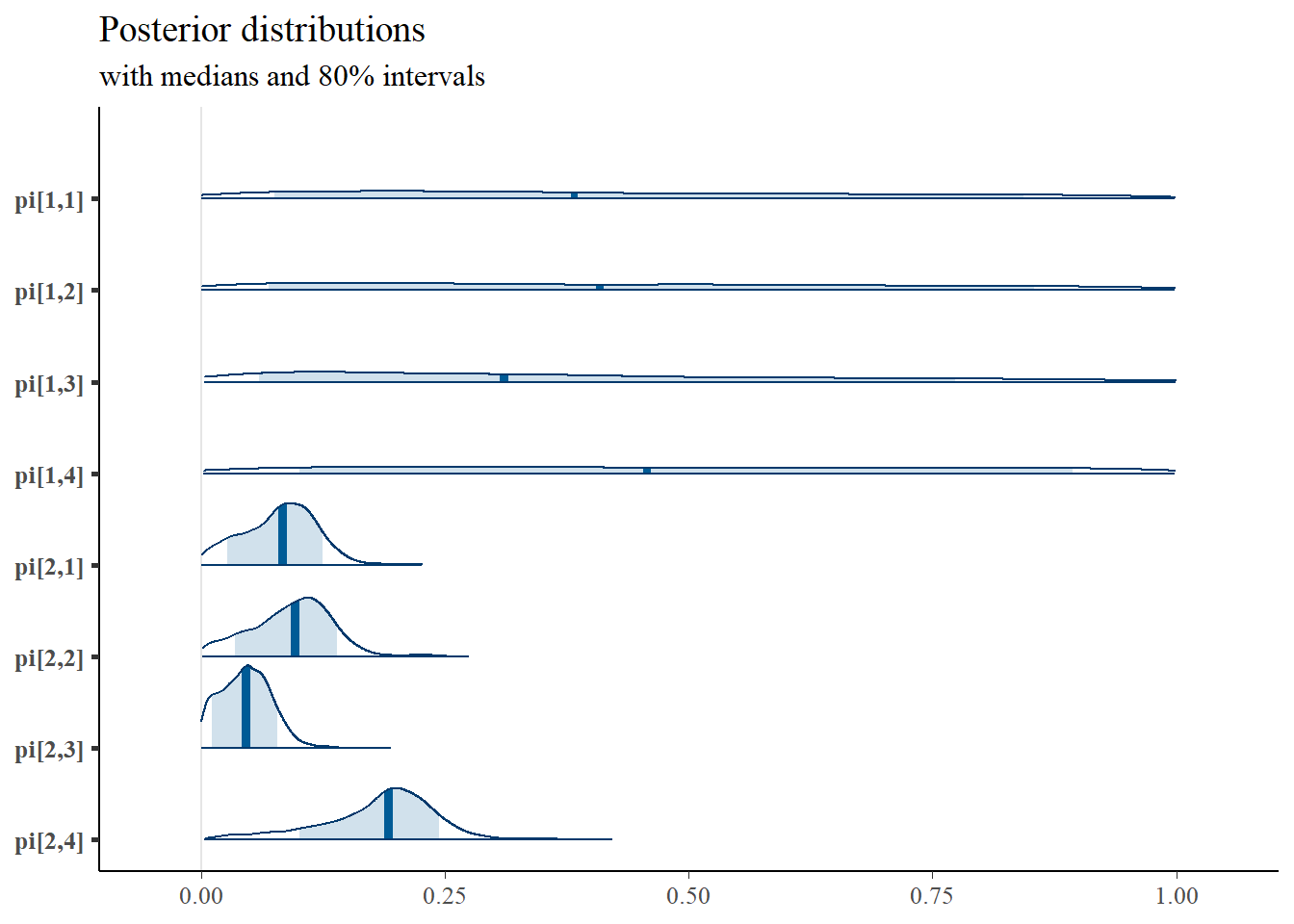
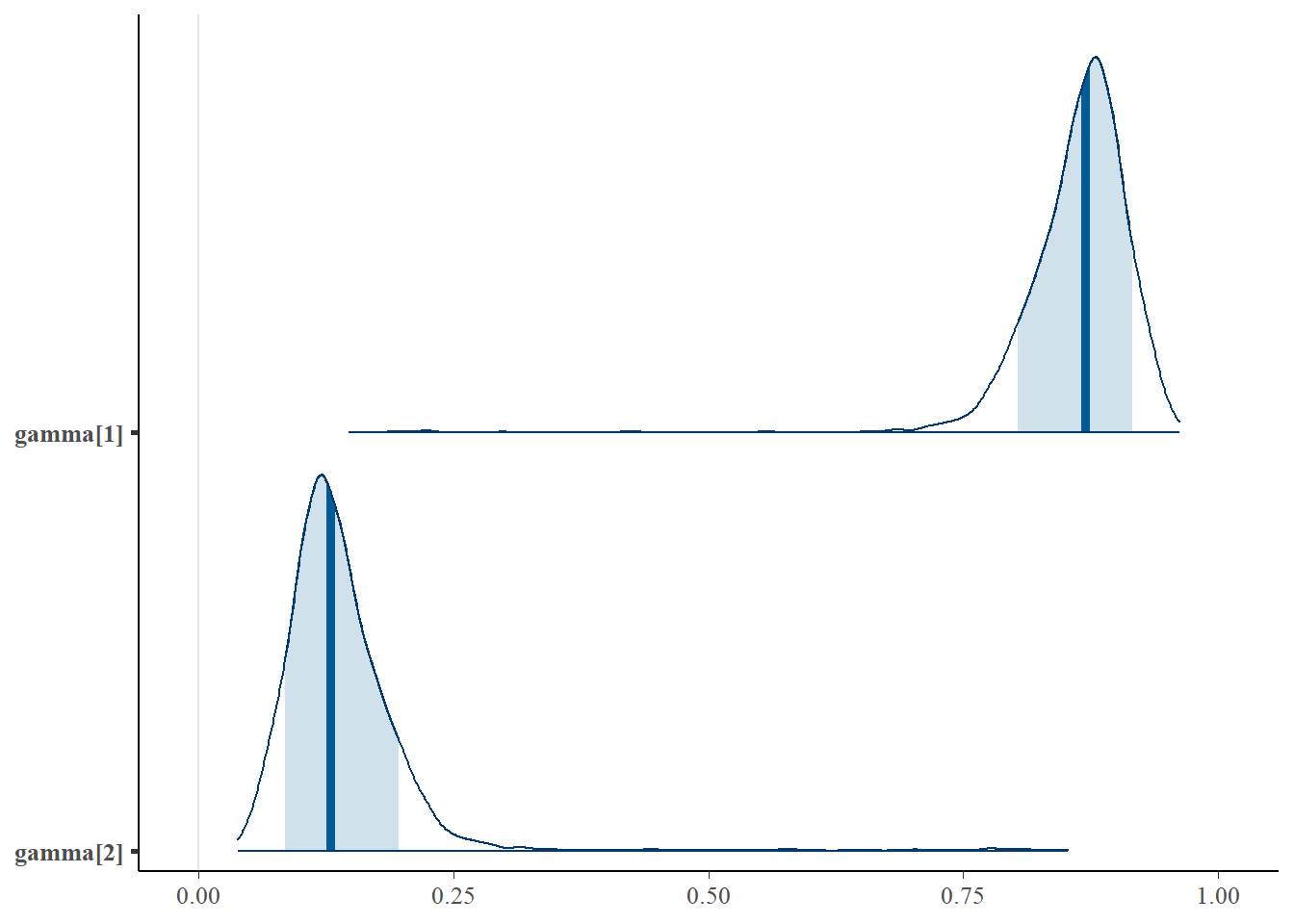
# plot the posterior density
plot.data <- as.matrix(fit)

plot_title <- ggtitle("Posterior distributions",
                      "with medians and 80% intervals")
mcmc_areas(
  plot.data,
  pars = paste0("gamma[",1:2,"]"),
  prob = 0.8) +
  plot_title
## Error in `select_parameters()`:
## ! Some 'pars' don't match parameter names: gamma[2] FALSE
mcmc_areas(
  plot.data,
  pars = c(paste0("pi[1,",1:4,"]"),paste0("pi[2,",1:4,"]")),
  prob = 0.8) +
  plot_title