8 Classical Test Theory
The traditional model specification for CTT is \[X = T + E,\] where \(X\) is the observed test/measure score, \(T\) is the truce score we wish to make inferences about, and \(E\) is the error. The true scores have population mean \(\mu_T\) and variance \(\sigma^2_T\). The errors for any individual are expected to be 0 on average, \(\mathbb{E}(E_i)=0\) with variance \(\sigma^2_E\). The errors are uncorrelated with the true score in the population, that is \[\mathbb{COV}(T, E) = \sigma_{TE} = \rho_{TE}\sigma_{T}\sigma_E = 0.\]
Some implications associated with the CTT model are:
The population mean of observed scores is the same as the true scores \[\mu_x = \mu_T.\]
The observed score variance can be decomposed into \[\begin{align*} \sigma^2_X &= \sigma^2_T + \sigma^2_E + 2\sigma_{TE}\\ &= \sigma^2_T + \sigma^2_E. \end{align*}\]
We can define the reliability in terms of the ratio of true score variance to observed score variance, that is \[\rho = \frac{\sigma^2_T}{\sigma^2_X} = \frac{\sigma^2_T}{\sigma^2_T + \sigma^2_E}.\]
An interesting approach to deriving estimates of true scores is to flip the traditional CTT model around so that we define the true score as a function of the observed score. This uses Kelley’s formula (Kelley 1923), \[\begin{align*} \hat{T}_i &= \rho x_i + (1-\rho)\mu_x\\ &= \mu_x + \rho (x_i - \mu_x), \end{align*}\] where \(\mu_x\) is the mean of the observed scores and \(\hat{T}_i\) is the estimated true score of individual \(i\). This is an interesting formula since there’s the notion about how to incorporate uncertainty into the estimation of the true score. The higher the uncertainty (lower the reliability) the less we weight the observed score and more we rely on the population mean as our estimate.
This has a very Bayesian feel to is, because it’s nearly identical to how we derive the posterior mean in a conjugate normal model (see p.158).
8.1 Example 1 - Known measurement model parameters with 1 measure
Here, we will discuss a simple CTT example where we assume that the measurement model parameters are known. This means we assume a value for \(\mu_t\), \(\sigma^2_T\), and \(\sigma^2_E\). We would nearly always need to estimate these quantities to provide an informed decision as to what these parameters should be.
This example using 3 observations (individuals) with 1 measure per individual. The DAG for this model is shown below.
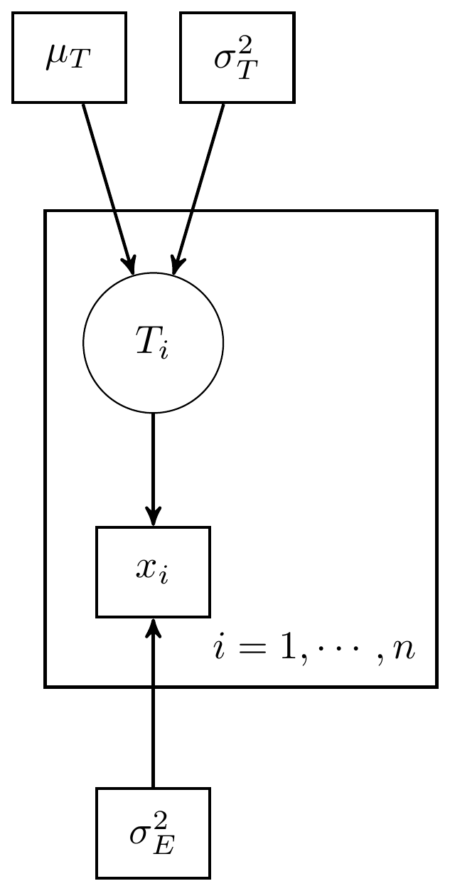
Figure 8.1: Simple CTT model with 1 measure and known measurement parameters
With a simply model specification using normal distributions as the underly probability functions.
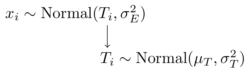
Figure 8.2: Model specification diagram for the known parameters CTT model
8.2 Example 1 - Stan
model_ctt1 <- '
data {
  int  N;
  real x[N];
  real muT;
  real sigmaT;
  real sigmaE;
}

parameters {
  real T[N];
}

model {
  for(i in 1:N){
    x[i] ~ normal(T[i], sigmaE);
    T[i] ~ normal(muT, sigmaT);
  }
}

'
# data must be in a list
mydata <- list(
  N=3,
  x=c(70, 80, 96),
  muT = 80,
  sigmaT = 6, #sqrt(36)
  sigmaE = 4 # sqrt(16)
)

# Next, need to fit the model
#   I have explicitly outlined some common parameters
fit <- stan(
  model_code = model_ctt1, # model code to be compiled
  data = mydata,          # my data
  chains = 4,             # number of Markov chains
  warmup = 1000,          # number of warm up iterations per chain
  iter = 5000,            # total number of iterations per chain
  cores = 4,              # number of cores (could use one per chain)
  refresh = 0             # no progress shown
)

# first get a basic breakdown of the posteriors
print(fit)
## Inference for Stan model: anon_model.
## 4 chains, each with iter=5000; warmup=1000; thin=1;
## post-warmup draws per chain=4000, total post-warmup draws=16000.
##
## mean se_mean sd 2.5% 25% 50% 75% 97.5% n_eff Rhat
## T[1] 73.13 0.02 3.31 66.66 70.88 73.12 75.36 79.66 18495 1
## T[2] 79.94 0.02 3.33 73.45 77.70 79.94 82.17 86.48 18747 1
## T[3] 91.10 0.03 3.33 84.61 88.81 91.10 93.36 97.74 15136 1
## lp__ -4.92 0.01 1.23 -8.14 -5.46 -4.61 -4.03 -3.53 8272 1
##
## Samples were drawn using NUTS(diag_e) at Sun Jun 19 17:32:47 2022.
## For each parameter, n_eff is a crude measure of effective sample size,
## and Rhat is the potential scale reduction factor on split chains (at
## convergence, Rhat=1).
# plot the posterior in a
#  95% probability interval
#  and 80% to contrast the dispersion
plot(fit)
## ci_level: 0.8 (80% intervals)## outer_level: 0.95 (95% intervals)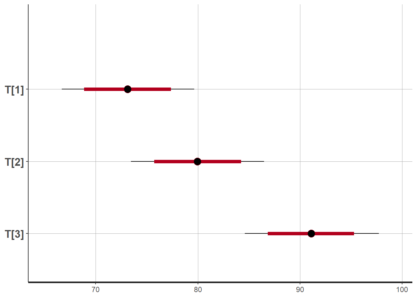
# Gelman-Rubin-Brooks Convergence Criterion
p1 <- ggs_grb(ggs(fit, family = "T")) +
   theme_bw() + theme(panel.grid = element_blank())
p1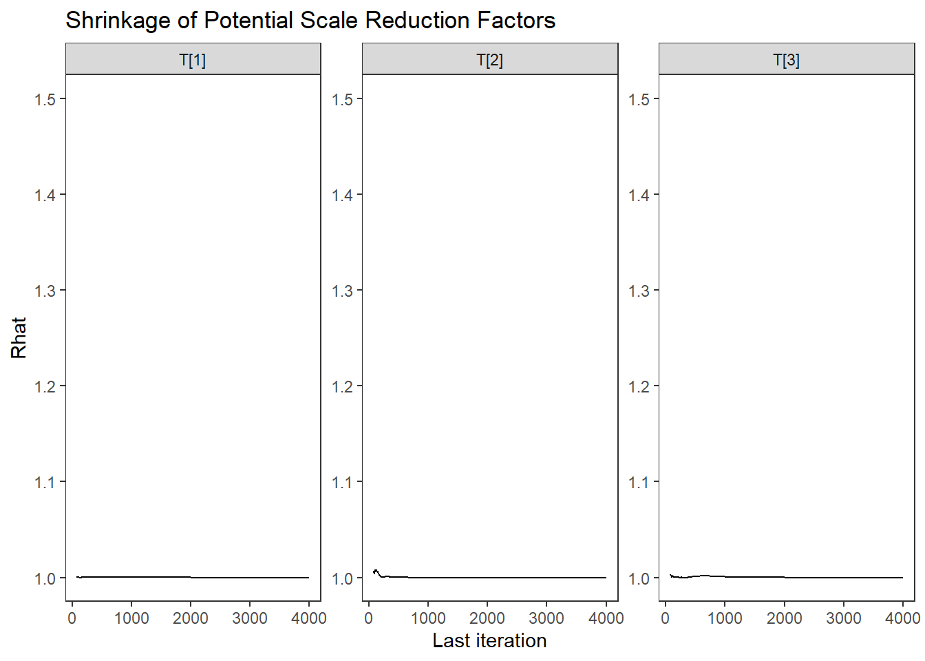
# autocorrelation
p1 <- ggs_autocorrelation(ggs(fit, family="T")) +
   theme_bw() + theme(panel.grid = element_blank())
p1 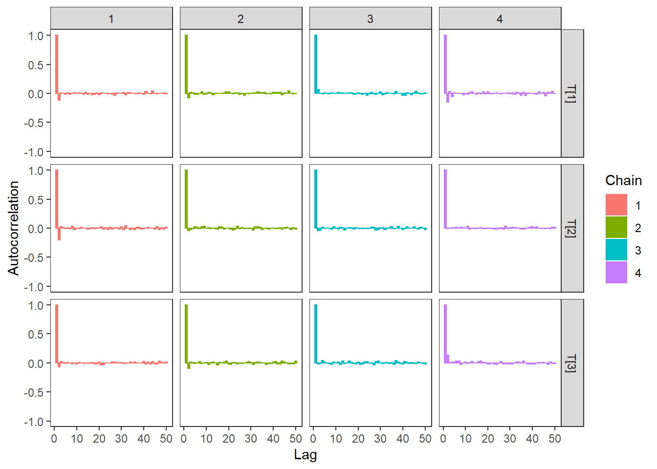
# plot the posterior density
plot.data <- as.matrix(fit)

plot_title <- ggtitle("Posterior distributions",
                      "with medians and 80% intervals")
mcmc_areas(
  plot.data,
  pars = c("T[1]","T[2]","T[3]"),
  prob = 0.8) +
  plot_title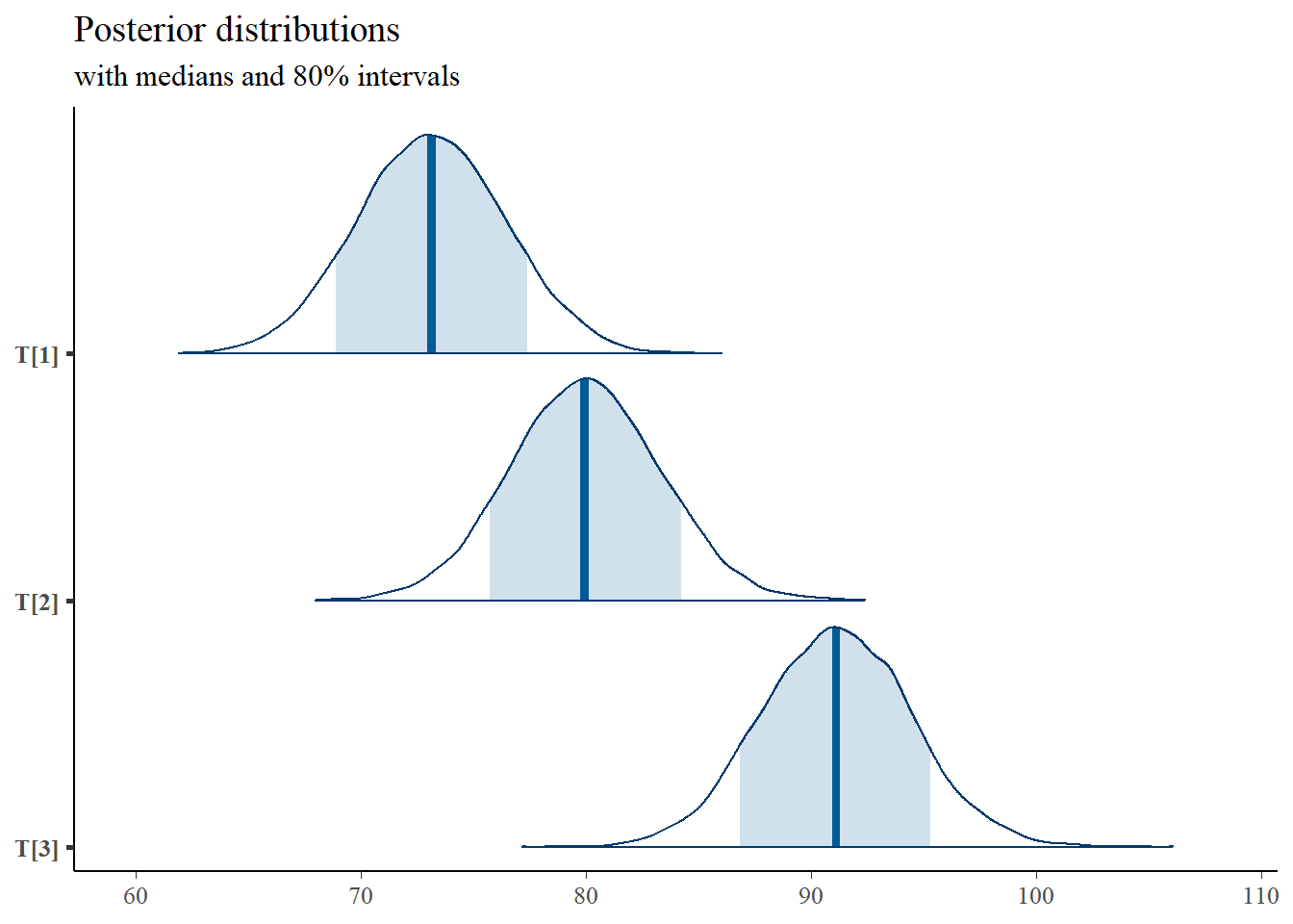
# I prefer a posterior plot that includes prior and MLE
# Expanded Posterior Plot
MLE <- mydata$x
prior_t <- function(x){dnorm(x, 80, 6)}
x.t<- seq(50.1, 100, 0.1)
prior.t <- data.frame(tr=x.t, dens.t = prior_t(x.t))
cols <- c("Posterior"="#0072B2", "Prior"="#E69F00", "MLE"= "black")#"#56B4E9", "#E69F00" "#CC79A7"
plot.data <- as.data.frame(plot.data)
p1 <- ggplot()+
  geom_density(data=plot.data,
               aes(x=`T[1]`, color="Posterior"))+
  geom_line(data=prior.t,
            aes(x=tr, y=dens.t, color="Prior"))+
  geom_vline(aes(xintercept=MLE[1], color="MLE"))+
  scale_color_manual(values=cols, name=NULL)+
  theme_bw()+
  theme(panel.grid = element_blank())

p2 <- ggplot()+
  geom_density(data=plot.data,
               aes(x=`T[2]`, color="Posterior"))+
  geom_line(data=prior.t,
            aes(x=tr, y=dens.t, color="Prior"))+
  geom_vline(aes(xintercept=MLE[2], color="MLE"))+
  scale_color_manual(values=cols, name=NULL)+
  theme_bw()+
  theme(panel.grid = element_blank())

p3 <- ggplot()+
  geom_density(data=plot.data,
               aes(x=`T[3]`, color="Posterior"))+
  geom_line(data=prior.t,
            aes(x=tr, y=dens.t, color="Prior"))+
  geom_vline(aes(xintercept=MLE[3], color="MLE"))+
  scale_color_manual(values=cols, name=NULL)+
  theme_bw()+
  theme(panel.grid = element_blank())

p1 + p2 + p3 + plot_layout(guides="collect")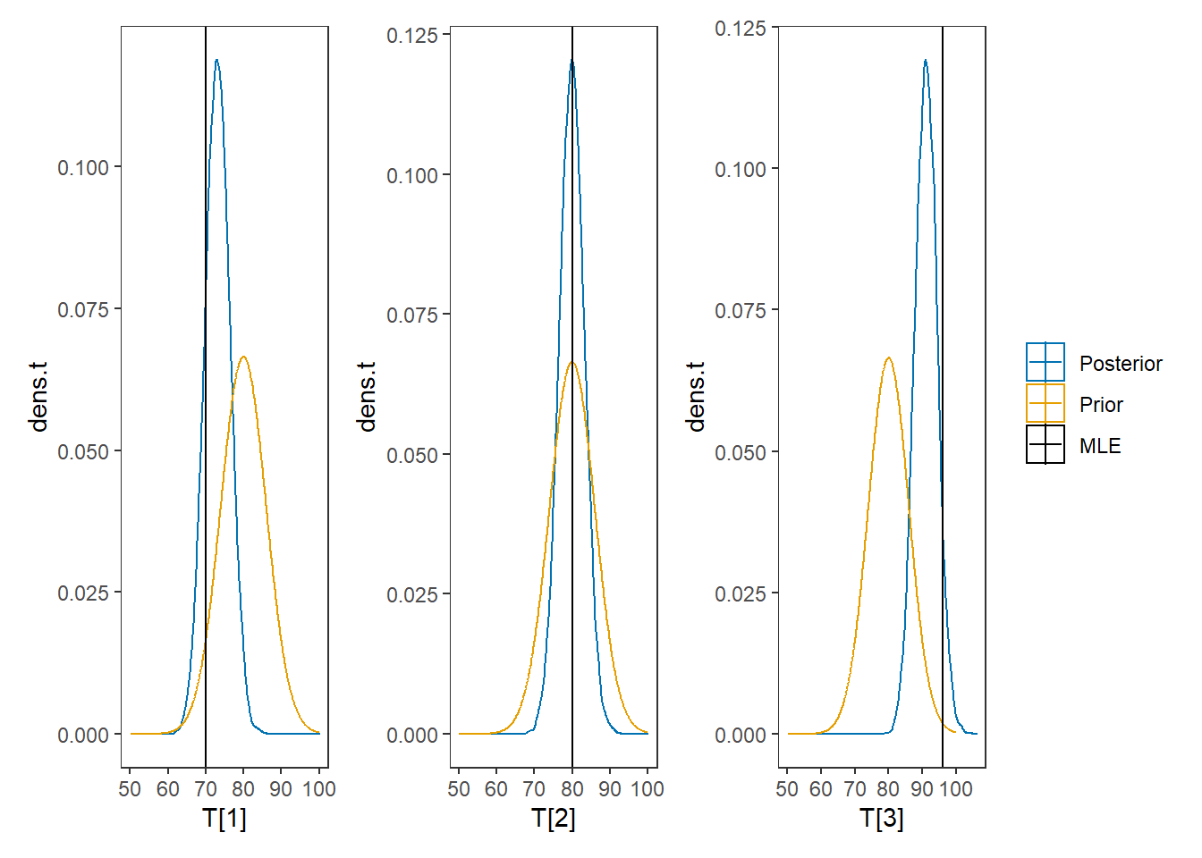
8.3 Example 1 - JAGS
# model code
jags.model.ctt1 <- function(){
   ############################################
     # CLASSICAL TEST THEORY MODEL
     # WITH KNOWN HYPERPARAMETERS
     #    TRUE SCORE MEAN, TRUE SCORE VARIANCE
     #    ERROR VARIANCE
     ############################################

     ############################################
     # KNOWN HYPERPARAMETERS
     ############################################
     mu.T <- 80               # Mean of the true scores
     sigma.squared.T <- 36    # Variance of the true scores
     sigma.squared.E <- 16    # Variance of the errors

     tau.T <- 1/sigma.squared.T   # Precision of the true scores
     tau.E <- 1/sigma.squared.E   # Precision of the errors


     ############################################
     # MODEL FOR TRUE SCORES AND OBSERVABLES
     ############################################

     for (i in 1:n) {
          T[i] ~ dnorm(mu.T, tau.T)     # Distribution of true scores
          x[i] ~ dnorm(T[i], tau.E)     # Distribution of observables
     }

}
# data
mydata <- list(
  n=3,
  x=c(70, 80, 96)
)

# starting values
start_values <- function(){
  list("T"=c(80,80,80))
}

# vector of all parameters to save
param_save <- c("T")

# fit model
fit <- jags(
  model.file=jags.model.ctt1,
  data=mydata,
  inits=start_values,
  parameters.to.save = param_save,
  n.iter=4000,
  n.burnin = 1000,
  n.chains = 4,
  n.thin=1,
  progress.bar = "none")
## Compiling model graph
## Resolving undeclared variables
## Allocating nodes
## Graph information:
## Observed stochastic nodes: 3
## Unobserved stochastic nodes: 3
## Total graph size: 13
##
## Initializing model
print(fit)## Inference for Bugs model at "C:/Users/noahp/AppData/Local/Temp/RtmpQR8sbs/model4544520665bc.txt", fit using jags,
## 4 chains, each with 4000 iterations (first 1000 discarded)
## n.sims = 12000 iterations saved
## mu.vect sd.vect 2.5% 25% 50% 75% 97.5% Rhat n.eff
## T[1] 73.086 3.292 66.649 70.841 73.088 75.308 79.526 1.001 7300
## T[2] 80.064 3.272 73.653 77.859 80.065 82.292 86.524 1.001 5500
## T[3] 91.045 3.341 84.470 88.763 91.061 93.306 97.453 1.001 12000
## deviance 18.005 2.932 14.208 15.784 17.399 19.551 25.289 1.001 12000
##
## For each parameter, n.eff is a crude measure of effective sample size,
## and Rhat is the potential scale reduction factor (at convergence, Rhat=1).
##
## DIC info (using the rule, pD = var(deviance)/2)
## pD = 4.3 and DIC = 22.3
## DIC is an estimate of expected predictive error (lower deviance is better).
# extract posteriors for all chains
jags.mcmc <- as.mcmc(fit)
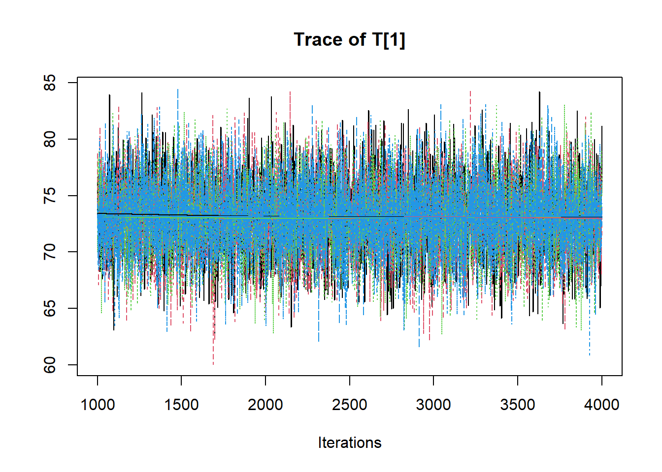
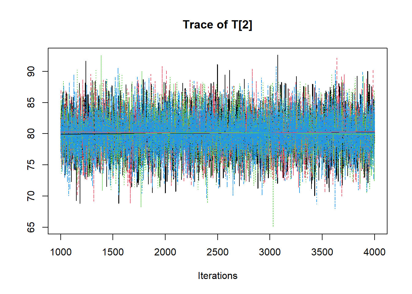
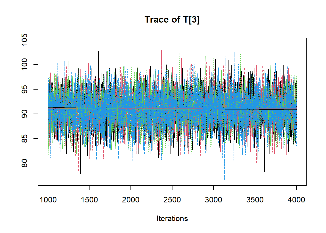
R2jags::traceplot(jags.mcmc)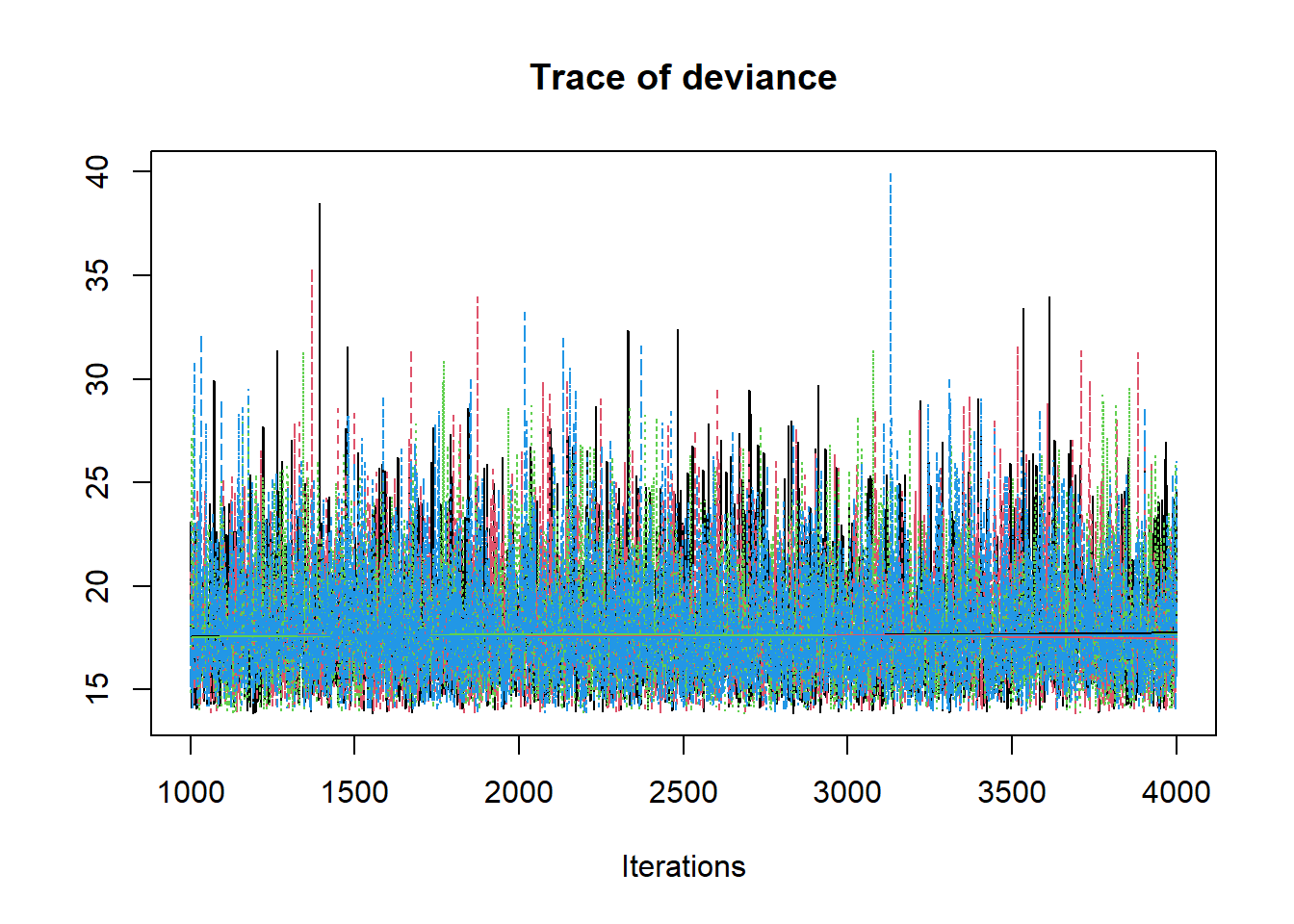
# gelman-rubin-brook
gelman.plot(jags.mcmc)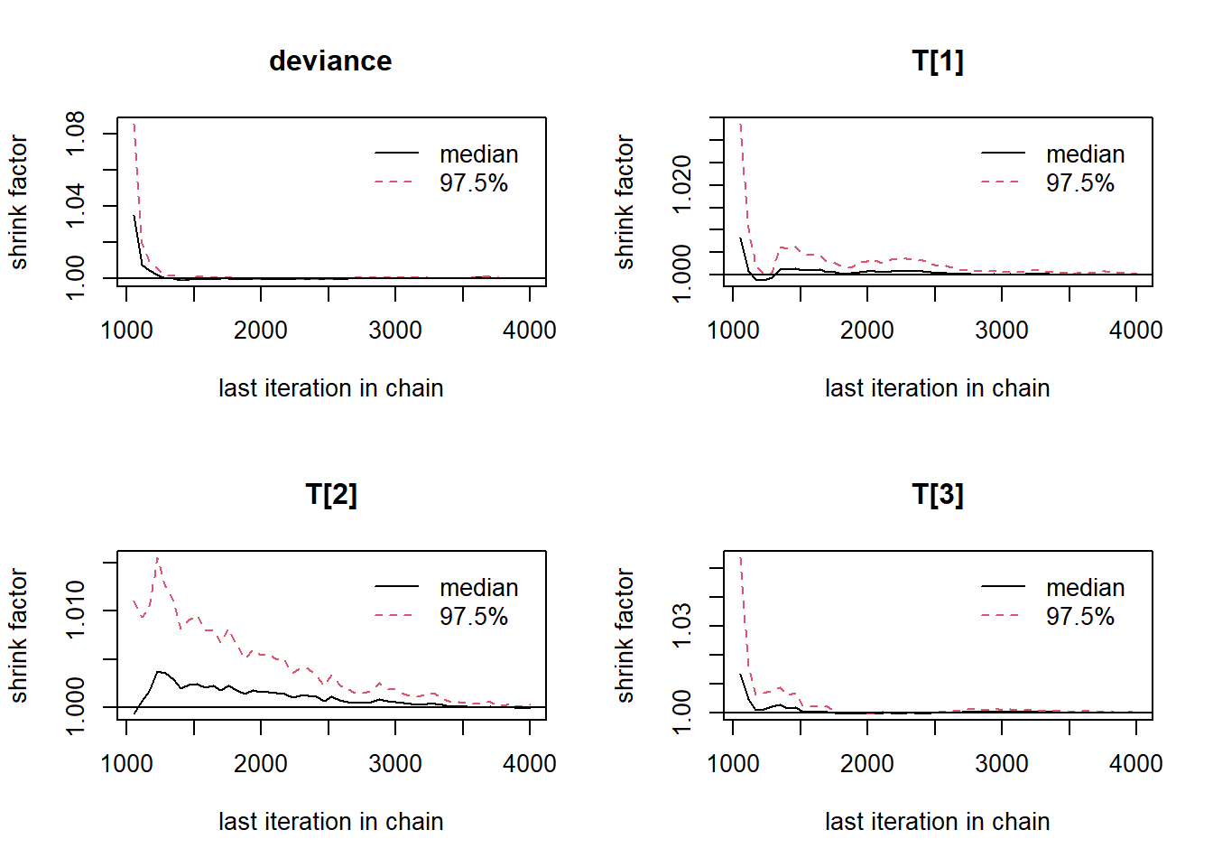
# convert to single data.frame for density plot
a <- colnames(as.data.frame(jags.mcmc[[1]]))
plot.data <- data.frame(as.matrix(jags.mcmc, chains=T, iters = T))
colnames(plot.data) <- c("chain", "iter", a)


plot_title <- ggtitle("Posterior distributions",
                      "with medians and 80% intervals")
mcmc_areas(
  plot.data,
  pars = c("T[1]", "T[2]", "T[3]"),
  prob = 0.8) +
  plot_title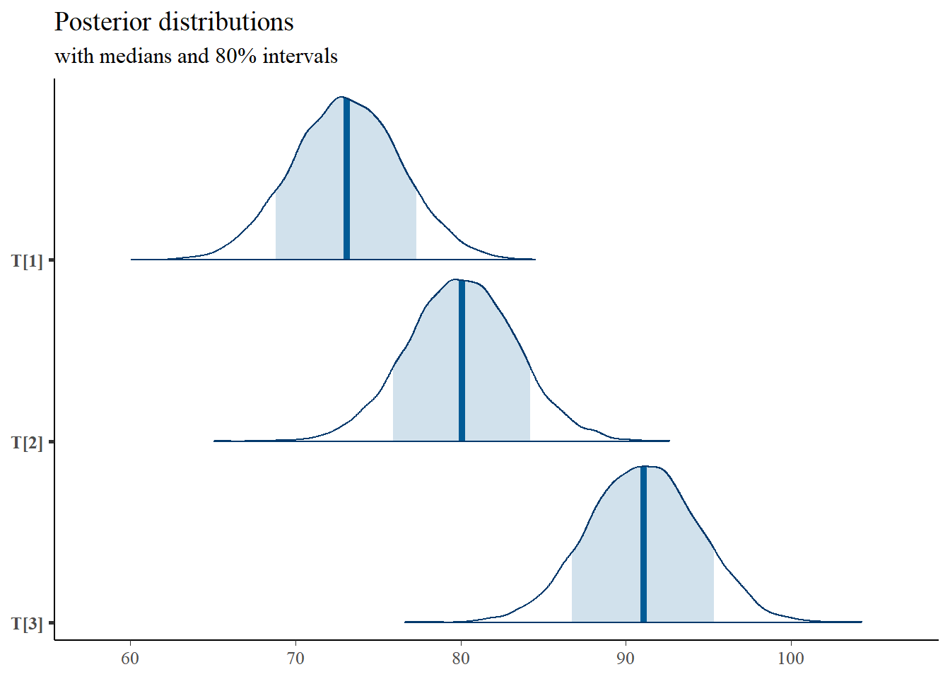
# I prefer a posterior plot that includes prior and MLE
MLE <- mydata$x
prior_t <- function(x){dnorm(x, 80, 6)}
x.t<- seq(50.1, 100, 0.1)
prior.t <- data.frame(tr=x.t, dens.t = prior_t(x.t))
cols <- c("Posterior"="#0072B2", "Prior"="#E69F00", "MLE"= "black")#"#56B4E9", "#E69F00" "#CC79A7"

p1 <- ggplot()+
  geom_density(data=plot.data,
               aes(x=`T[1]`, color="Posterior"))+
  geom_line(data=prior.t,
            aes(x=tr, y=dens.t, color="Prior"))+
  geom_vline(aes(xintercept=MLE[1], color="MLE"))+
  scale_color_manual(values=cols, name=NULL)+
  theme_bw()+
  theme(panel.grid = element_blank())

p2 <- ggplot()+
  geom_density(data=plot.data,
               aes(x=`T[2]`, color="Posterior"))+
  geom_line(data=prior.t,
            aes(x=tr, y=dens.t, color="Prior"))+
  geom_vline(aes(xintercept=MLE[2], color="MLE"))+
  scale_color_manual(values=cols, name=NULL)+
  theme_bw()+
  theme(panel.grid = element_blank())

p3 <- ggplot()+
  geom_density(data=plot.data,
               aes(x=`T[3]`, color="Posterior"))+
  geom_line(data=prior.t,
            aes(x=tr, y=dens.t, color="Prior"))+
  geom_vline(aes(xintercept=MLE[3], color="MLE"))+
  scale_color_manual(values=cols, name=NULL)+
  theme_bw()+
  theme(panel.grid = element_blank())

p1 + p2 + p3 + plot_layout(guides="collect")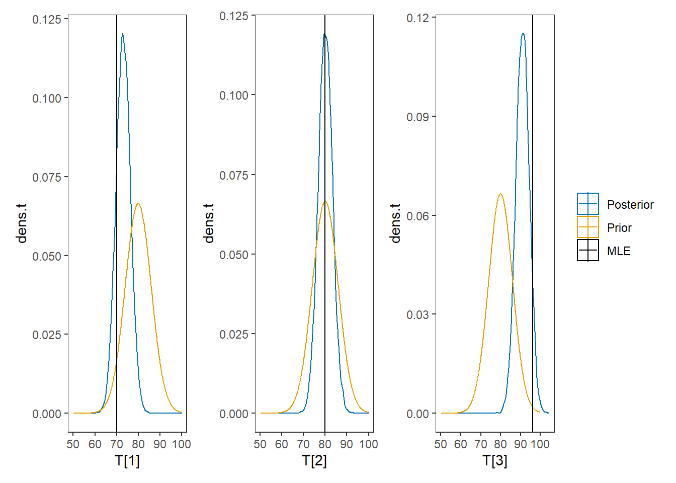
8.4 Example 2 - Known Measurement Model with Multiple Measures
Here, the only thing that changes from the first example is that now we have multiple observations per individual. We can think of this as if we could administer a test (or parallel tests) repeatedly without learning occuring. The DAG and model-specification change to:
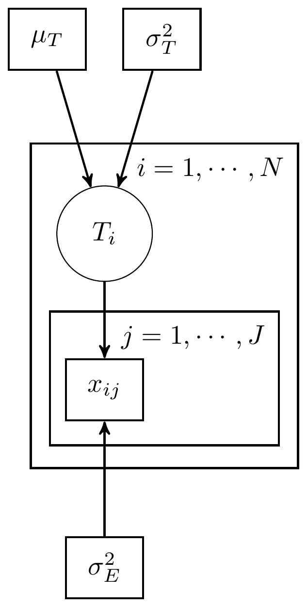
Figure 8.3: Simple CTT model with known measurement parameters and multiple measures
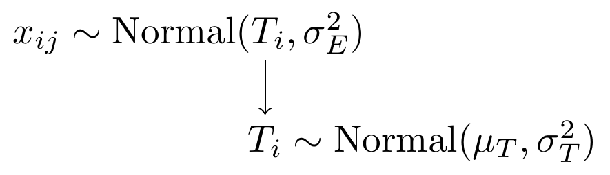
Figure 8.4: Model specification diagram for the known parameters CTT model and multiple measures
8.5 Example 2 - Stan
model_ctt2 <- '
data {
  int  N;
  int  J;
  matrix[N, J] X;
  real muT;
  real sigmaT;
  real sigmaE;
}

parameters {
  real T[N];
}

model {
  for(i in 1:N){
    T[i] ~ normal(muT, sigmaT);
    for(j in 1:J){
      X[i, j] ~ normal(T[i], sigmaE);
    }
  }
}

'
# data must be in a list
mydata <- list(
  N = 10, J = 5,
  X = matrix(
    c(80, 77, 80, 73, 73,
      83, 79, 78, 78, 77,
      85, 77, 88, 81, 80,
      76, 76, 76, 78, 67,
      70, 69, 73, 71, 77,
      87, 89, 92, 91, 87,
      76, 75, 79, 80, 75,
      86, 75, 80, 80, 82,
      84, 79, 79, 77, 82,
      96, 85, 91, 87, 90),
    ncol=5, nrow=10, byrow=T),
  muT = 80,
  sigmaT = 6, #sqrt(36)
  sigmaE = 4 # sqrt(16)
)

# initial values
start_values <- function(){
  list(T=c(80,80,80,80,80,80,80,80,80,80))
}

# Next, need to fit the model
#   I have explicitly outlined some common parameters
fit <- stan(
  model_code = model_ctt2, # model code to be compiled
  data = mydata,          # my data
  init = start_values,    # starting values
  chains = 4,             # number of Markov chains
  warmup = 1000,          # number of warm up iterations per chain
  iter = 5000,            # total number of iterations per chain
  cores = 4,              # number of cores (could use one per chain)
  refresh = 0             # no progress shown
)

# first get a basic breakdown of the posteriors
print(fit)
## Inference for Stan model: anon_model.
## 4 chains, each with iter=5000; warmup=1000; thin=1;
## post-warmup draws per chain=4000, total post-warmup draws=16000.
##
## mean se_mean sd 2.5% 25% 50% 75% 97.5% n_eff Rhat
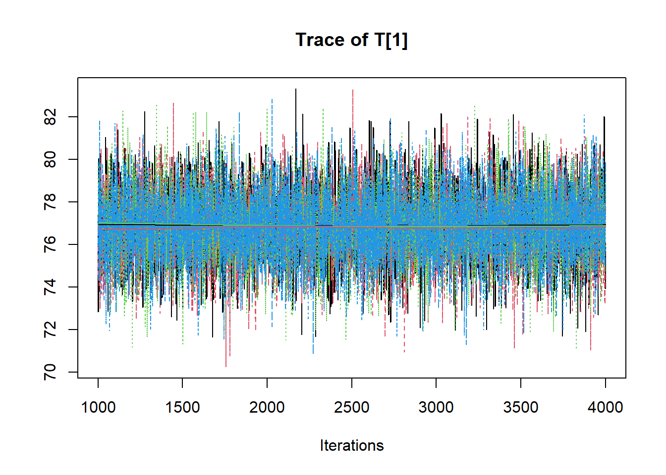
## T[1] 76.88 0.01 1.72 73.47 75.72 76.90 78.03 80.21 31735 1
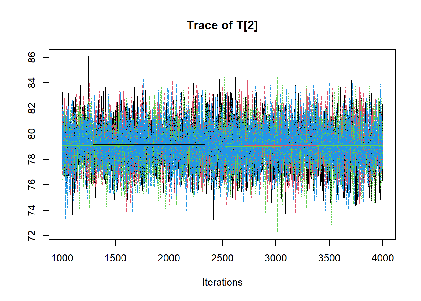
## T[2] 79.08 0.01 1.73 75.69 77.93 79.06 80.22 82.47 29246 1
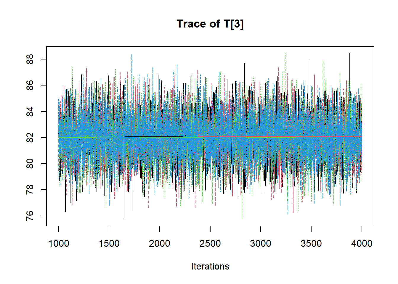
## T[3] 82.01 0.01 1.72 78.65 80.84 82.01 83.20 85.40 29176 1
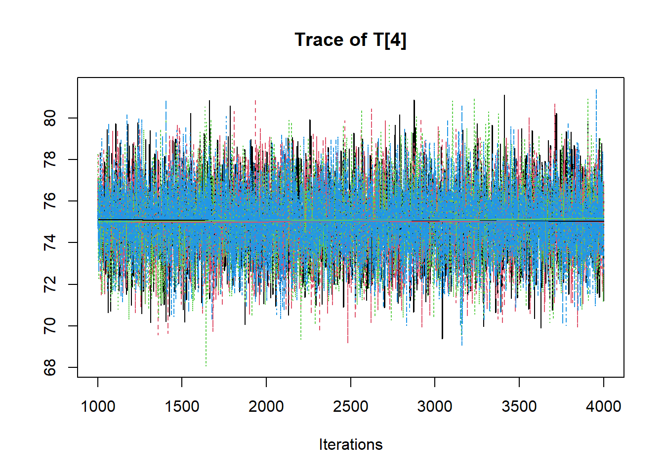
## T[4] 75.05 0.01 1.71 71.72 73.89 75.06 76.22 78.41 28913 1
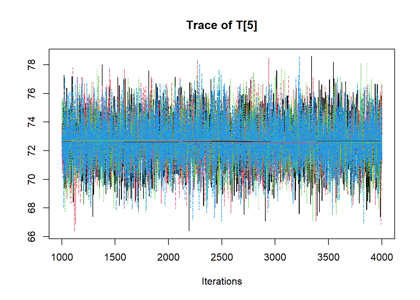
## T[5] 72.66 0.01 1.71 69.29 71.52 72.65 73.82 76.04 29610 1
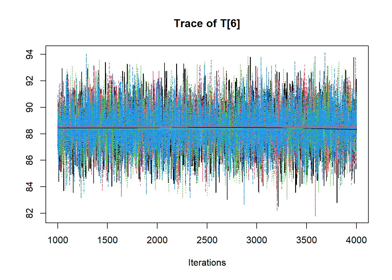
## T[6] 88.44 0.01 1.70 85.12 87.32 88.44 89.57 91.76 28373 1
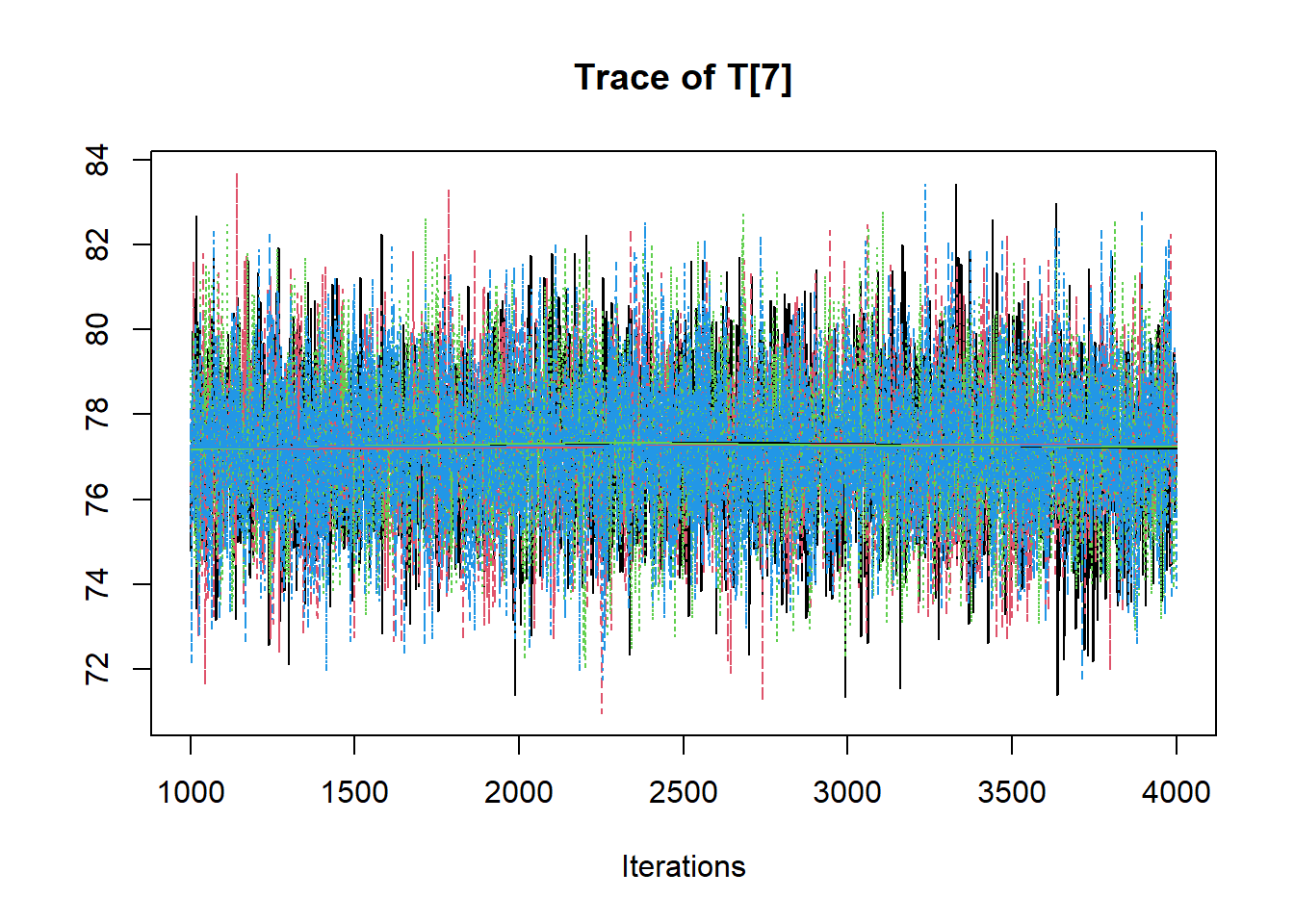
## T[7] 77.24 0.01 1.70 73.91 76.08 77.24 78.38 80.57 30229 1
## T[8] 80.56 0.01 1.69 77.25 79.43 80.56 81.72 83.84 28684 1
## T[9] 80.19 0.01 1.70 76.86 79.04 80.19 81.33 83.53 26627 1
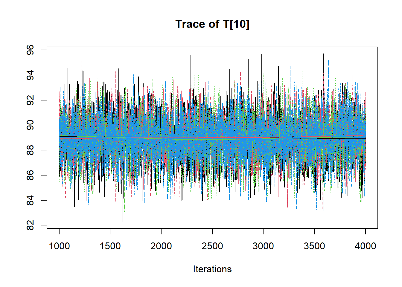
## T[10] 89.00 0.01 1.74 85.60 87.83 88.99 90.18 92.39 29996 1
## lp__ -23.47 0.03 2.22 -28.78 -24.72 -23.16 -21.87 -20.10 7486 1
##
## Samples were drawn using NUTS(diag_e) at Sun Jun 19 17:33:57 2022.
## For each parameter, n_eff is a crude measure of effective sample size,
## and Rhat is the potential scale reduction factor on split chains (at
## convergence, Rhat=1).
# plot the posterior in a
#  95% probability interval
#  and 80% to contrast the dispersion
plot(fit)
## ci_level: 0.8 (80% intervals)## outer_level: 0.95 (95% intervals)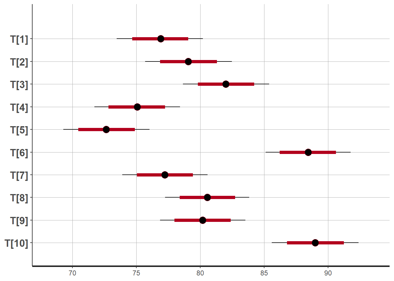
# Gelman-Rubin-Brooks Convergence Criterion
p1 <- ggs_grb(ggs(fit, family = "T")) +
   theme_bw() + theme(panel.grid = element_blank())
p1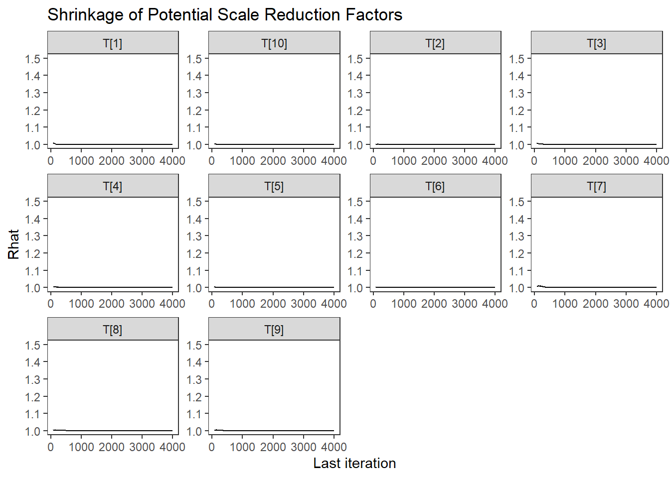
# autocorrelation
p1 <- ggs_autocorrelation(ggs(fit, family="T")) +
   theme_bw() + theme(panel.grid = element_blank())
p1 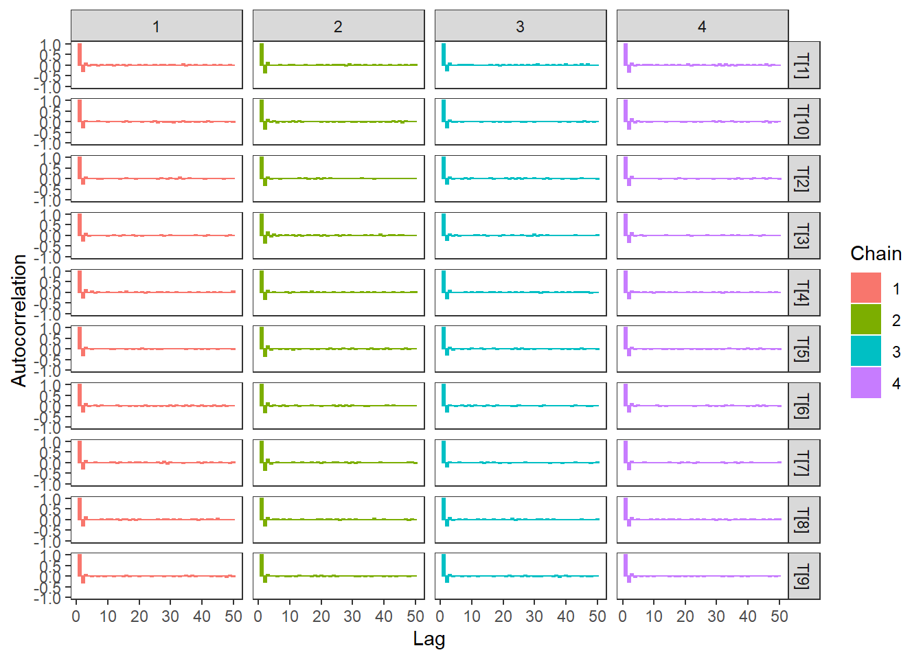
# plot the posterior density
plot.data <- as.matrix(fit)

plot_title <- ggtitle("Posterior distributions",
                      "with medians and 80% intervals")
mcmc_areas(
  plot.data,
  pars = paste0("T[",1:10,"]"),
  prob = 0.8) +
  plot_title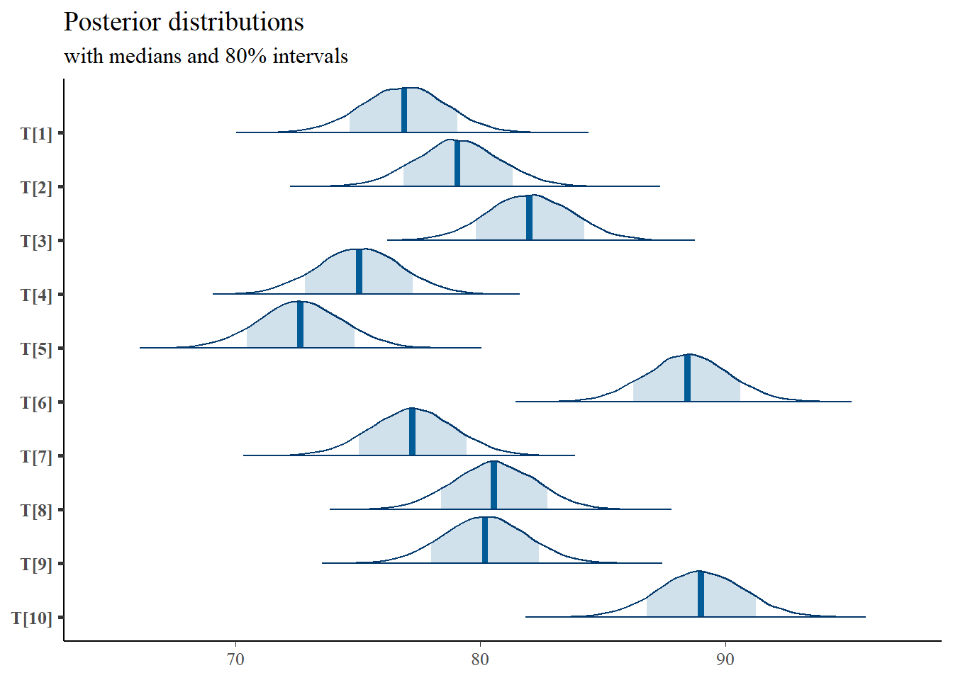
# I prefer a posterior plot that includes prior and MLE
# Expanded Posterior Plot
MLE <- rowMeans(mydata$X)
prior_t <- function(x){dnorm(x, 80, 6)}
x.t<- seq(50.1, 100, 0.1)
prior.t <- data.frame(tr=x.t, dens.t = prior_t(x.t))
cols <- c("Posterior"="#0072B2", "Prior"="#E69F00", "MLE"= "black")#"#56B4E9", "#E69F00" "#CC79A7"
plot.data <- as.data.frame(plot.data)
p1 <- ggplot()+
  geom_density(data=plot.data,
               aes(x=`T[1]`, color="Posterior"))+
  geom_line(data=prior.t,
            aes(x=tr, y=dens.t, color="Prior"))+
  geom_vline(aes(xintercept=MLE[1], color="MLE"))+
  scale_color_manual(values=cols, name=NULL)+
  theme_bw()+
  theme(panel.grid = element_blank())

p2 <- ggplot()+
  geom_density(data=plot.data,
               aes(x=`T[2]`, color="Posterior"))+
  geom_line(data=prior.t,
            aes(x=tr, y=dens.t, color="Prior"))+
  geom_vline(aes(xintercept=MLE[2], color="MLE"))+
  scale_color_manual(values=cols, name=NULL)+
  theme_bw()+
  theme(panel.grid = element_blank())

p3 <- ggplot()+
  geom_density(data=plot.data,
               aes(x=`T[5]`, color="Posterior"))+
  geom_line(data=prior.t,
            aes(x=tr, y=dens.t, color="Prior"))+
  geom_vline(aes(xintercept=MLE[5], color="MLE"))+
  scale_color_manual(values=cols, name=NULL)+
  theme_bw()+
  theme(panel.grid = element_blank())

p4 <- ggplot()+
  geom_density(data=plot.data,
               aes(x=`T[10]`, color="Posterior"))+
  geom_line(data=prior.t,
            aes(x=tr, y=dens.t, color="Prior"))+
  geom_vline(aes(xintercept=MLE[10], color="MLE"))+
  scale_color_manual(values=cols, name=NULL)+
  theme_bw()+
  theme(panel.grid = element_blank())


p1 + p2 + p3 + p4 + plot_layout(guides="collect")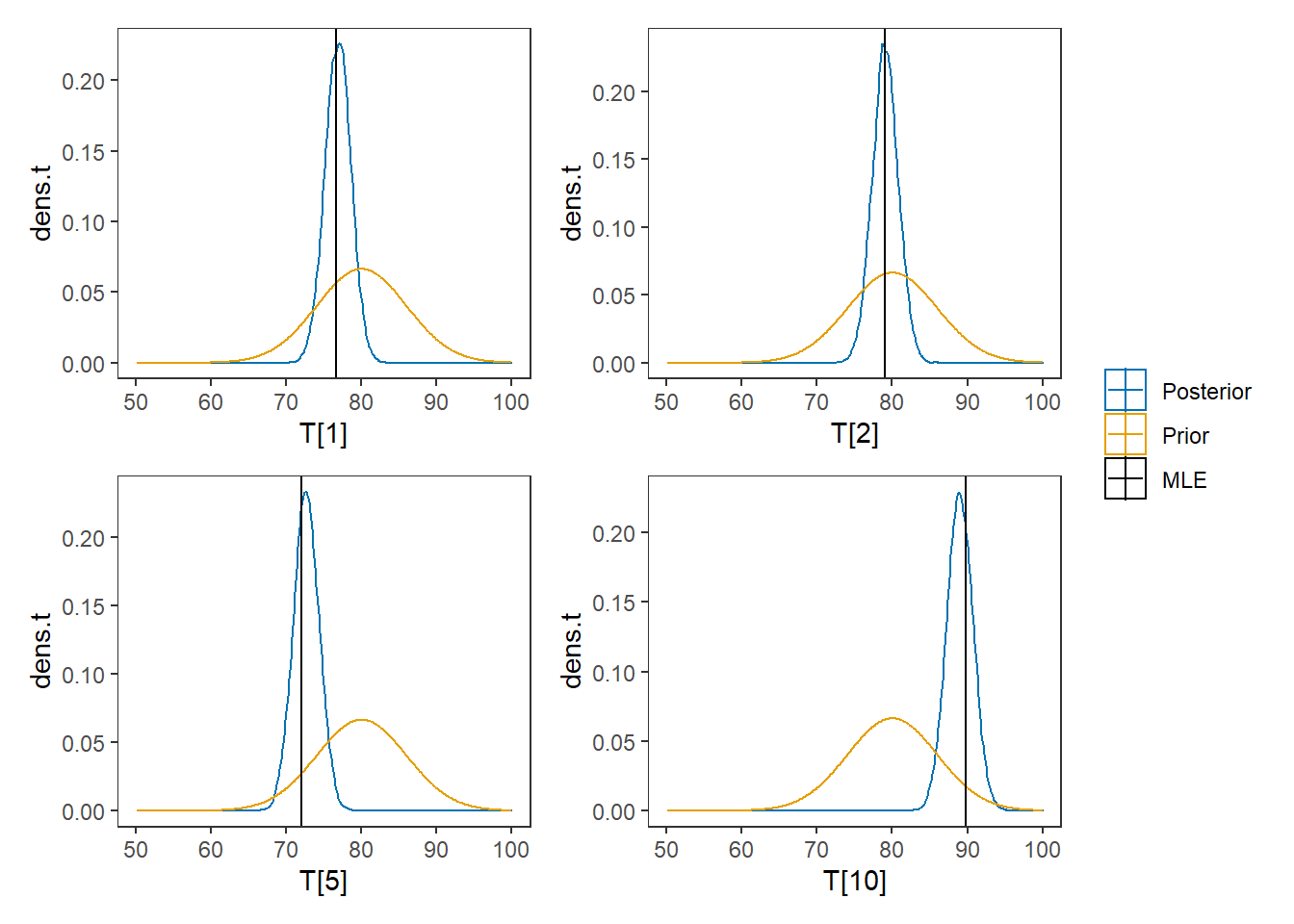
8.6 Example 2 - JAGS
# model code
jags.model.ctt2 <- function(){
   ############################################
     # CLASSICAL TEST THEORY
     # WITH KNOWN
     #    TRUE SCORE MEAN, TRUE SCORE VARIANCE
     #    ERROR VARIANCE
     ############################################

     ############################################
     # KNOWN HYPERPARAMETERS
     ############################################
     mu.T <- 80               # Mean of the true scores
     sigma.squared.T <- 36    # Variance of the true scores
     sigma.squared.E <- 16    # Variance of the errors

     tau.T <- 1/sigma.squared.T   # Precision of the true scores
     tau.E <- 1/sigma.squared.E   # Precision of the errors


     ############################################
     # MODEL FOR TRUE SCORES AND OBSERVABLES
     ############################################

     for (i in 1:N) {
        T[i] ~ dnorm(mu.T, tau.T)     # Distribution of true scores
        for(j in 1:J){
          x[i, j] ~ dnorm(T[i], tau.E)     # Distribution of observables
        }
     }

}
# data
mydata <- list(
  N = 10, J = 5,
  x = matrix(
    c(80, 77, 80, 73, 73,
      83, 79, 78, 78, 77,
      85, 77, 88, 81, 80,
      76, 76, 76, 78, 67,
      70, 69, 73, 71, 77,
      87, 89, 92, 91, 87,
      76, 75, 79, 80, 75,
      86, 75, 80, 80, 82,
      84, 79, 79, 77, 82,
      96, 85, 91, 87, 90),
    ncol=5, nrow=10, byrow=T)
)

# starting values
start_values <- function(){
  list("T"=rep(80,10))
}

# vector of all parameters to save
param_save <- c("T")

# fit model
fit <- jags(
  model.file=jags.model.ctt2,
  data=mydata,
  inits=start_values,
  parameters.to.save = param_save,
  n.iter=4000,
  n.burnin = 1000,
  n.chains = 4,
  n.thin=1,
  progress.bar = "none")
## Compiling model graph
## Resolving undeclared variables
## Allocating nodes
## Graph information:
## Observed stochastic nodes: 50
## Unobserved stochastic nodes: 10
## Total graph size: 68
##
## Initializing model
print(fit)## Inference for Bugs model at "C:/Users/noahp/AppData/Local/Temp/RtmpQR8sbs/model4544135343d3.txt", fit using jags,
## 4 chains, each with 4000 iterations (first 1000 discarded)
## n.sims = 12000 iterations saved
## mu.vect sd.vect 2.5% 25% 50% 75% 97.5% Rhat n.eff
## T[1] 76.858 1.693 73.521 75.712 76.845 77.982 80.164 1.001 4200
## T[2] 79.090 1.729 75.747 77.933 79.089 80.257 82.522 1.001 12000
## T[3] 82.028 1.700 78.704 80.860 82.031 83.173 85.338 1.001 12000
## T[4] 75.056 1.725 71.642 73.891 75.053 76.205 78.492 1.001 9800
## T[5] 72.654 1.695 69.363 71.489 72.633 73.808 75.984 1.001 12000
## T[6] 88.455 1.710 85.055 87.304 88.445 89.603 91.821 1.002 3100
## T[7] 77.261 1.702 73.905 76.145 77.252 78.399 80.587 1.001 12000
## T[8] 80.560 1.720 77.240 79.401 80.547 81.720 83.941 1.001 12000
## T[9] 80.211 1.707 76.886 79.050 80.219 81.373 83.565 1.001 3900
## T[10] 88.983 1.707 85.609 87.848 88.993 90.136 92.290 1.001 12000
## deviance 269.583 4.346 263.043 266.415 268.950 271.992 279.779 1.001 6800
##
## For each parameter, n.eff is a crude measure of effective sample size,
## and Rhat is the potential scale reduction factor (at convergence, Rhat=1).
##
## DIC info (using the rule, pD = var(deviance)/2)
## pD = 9.4 and DIC = 279.0
## DIC is an estimate of expected predictive error (lower deviance is better).
# extract posteriors for all chains
jags.mcmc <- as.mcmc(fit)
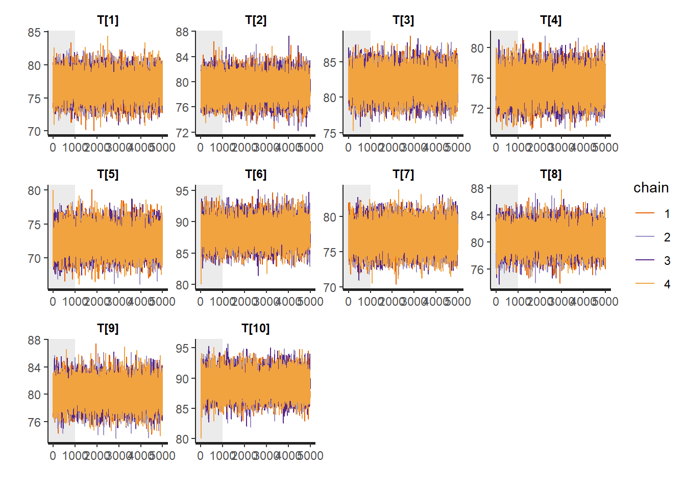
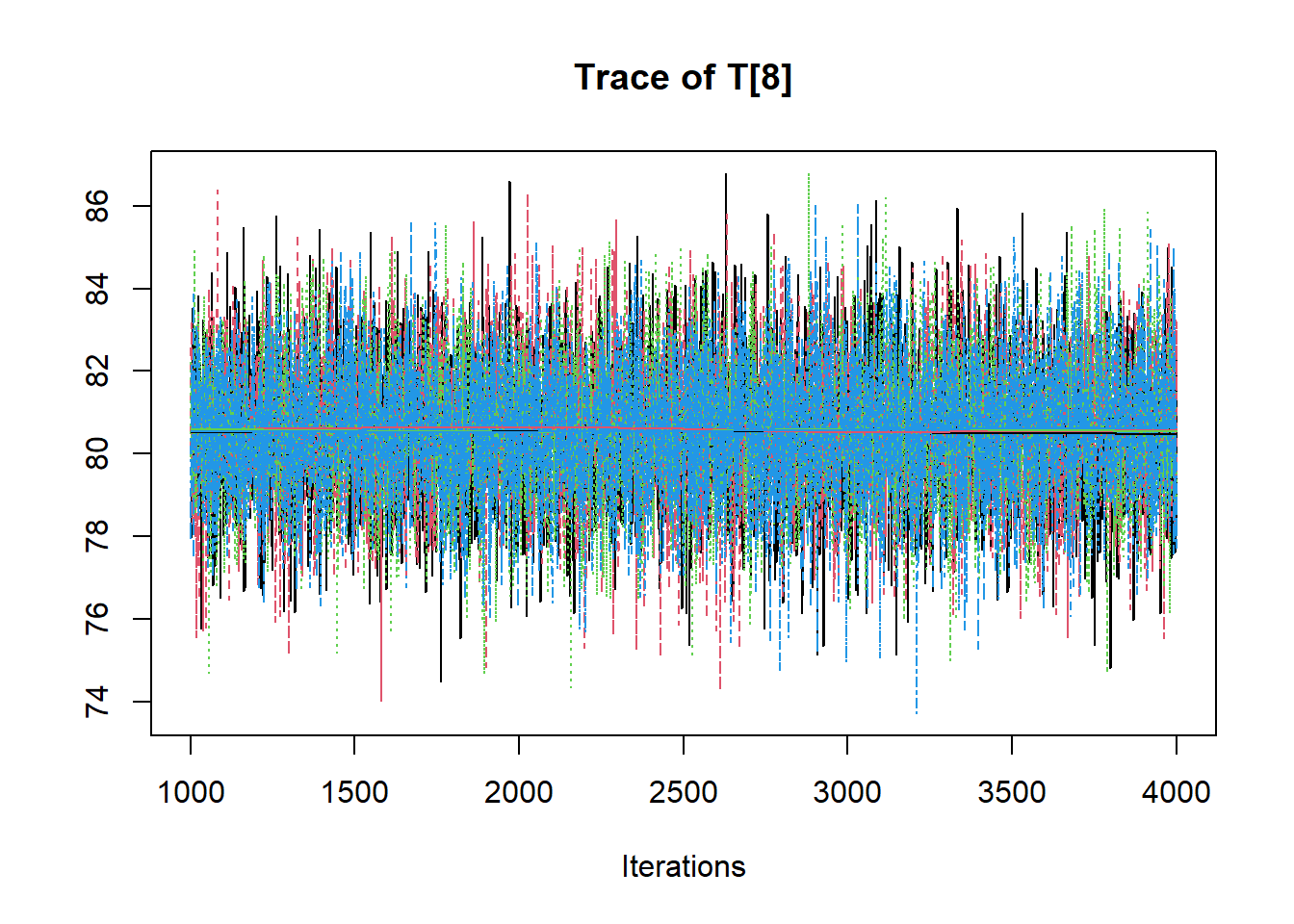
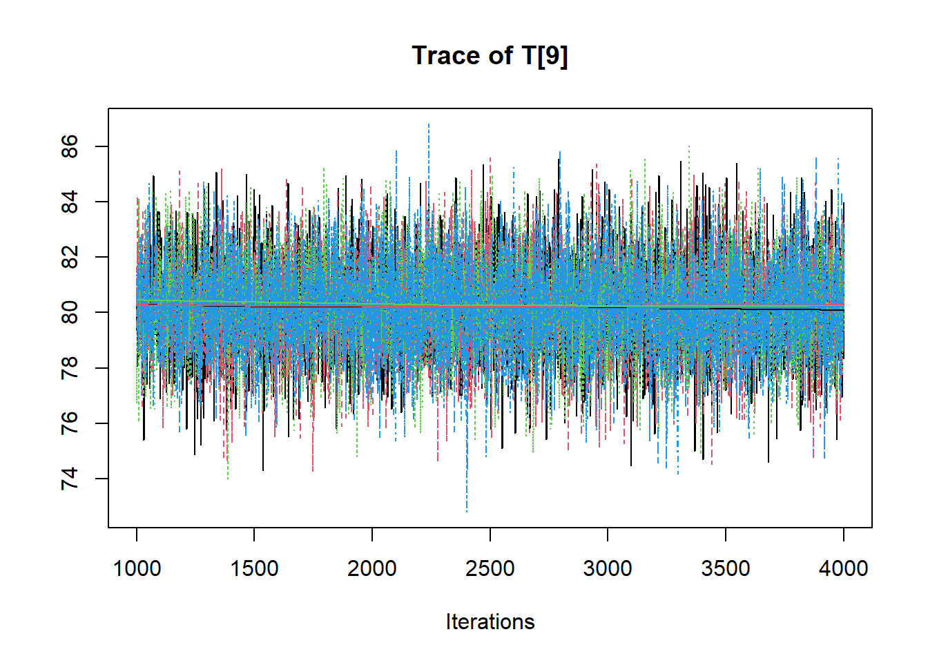
R2jags::traceplot(jags.mcmc)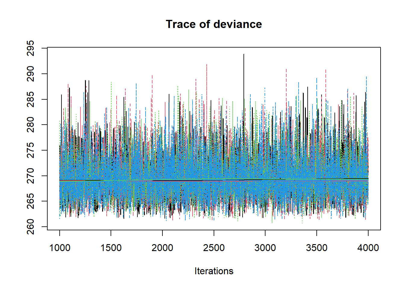
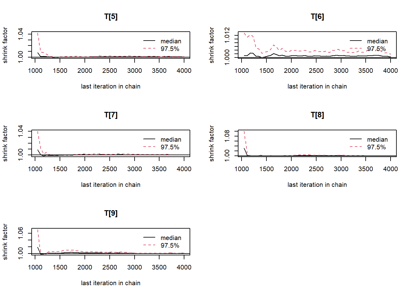
# gelman-rubin-brook
gelman.plot(jags.mcmc)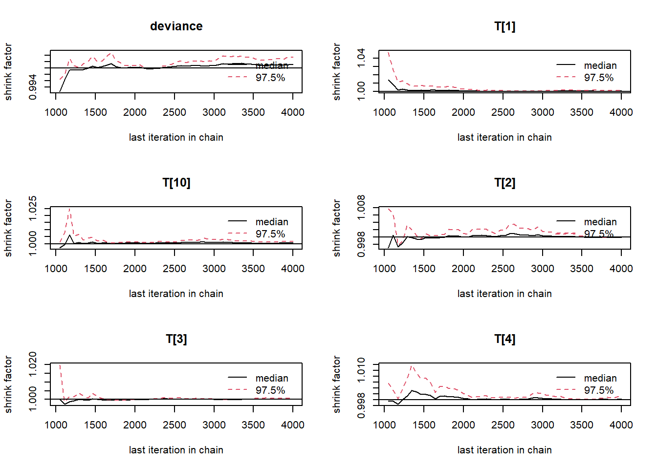
# convert to single data.frame for density plot
a <- colnames(as.data.frame(jags.mcmc[[1]]))
plot.data <- data.frame(as.matrix(jags.mcmc, chains=T, iters = T))
colnames(plot.data) <- c("chain", "iter", a)


plot_title <- ggtitle("Posterior distributions",
                      "with medians and 80% intervals")
mcmc_areas(
  plot.data,
  pars = c("T[1]", "T[2]", "T[3]"),
  prob = 0.8) +
  plot_title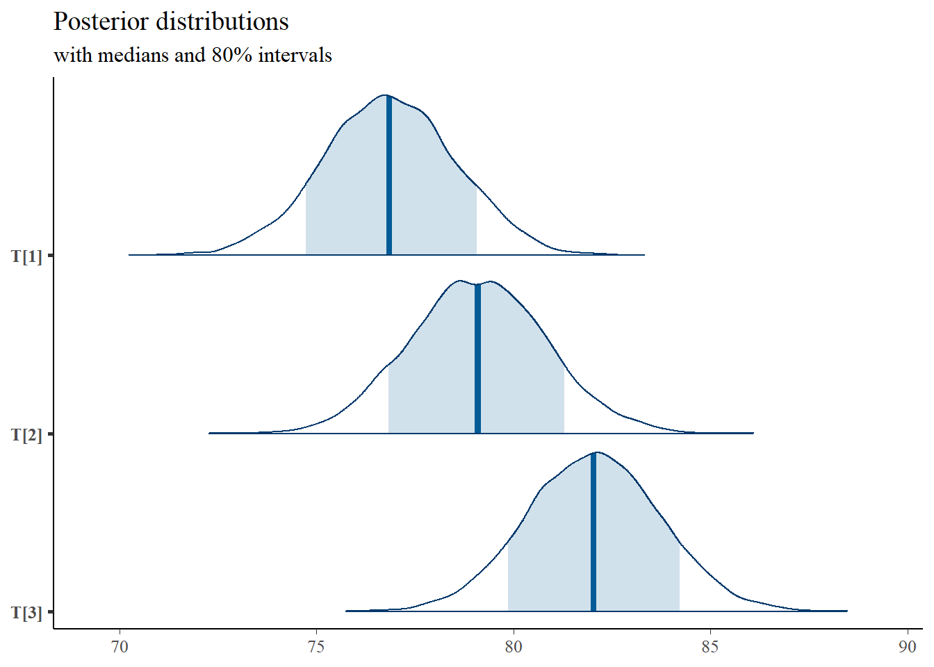
# I prefer a posterior plot that includes prior and MLE
MLE <- rowMeans(mydata$X)
## Error in rowMeans(mydata$X): 'x' must be an array of at least two dimensions
prior_t <- function(x){dnorm(x, 80, 6)}
x.t<- seq(50.1, 100, 0.1)
prior.t <- data.frame(tr=x.t, dens.t = prior_t(x.t))
cols <- c("Posterior"="#0072B2", "Prior"="#E69F00", "MLE"= "black")#"#56B4E9", "#E69F00" "#CC79A7"

p1 <- ggplot()+
  geom_density(data=plot.data,
               aes(x=`T[1]`, color="Posterior"))+
  geom_line(data=prior.t,
            aes(x=tr, y=dens.t, color="Prior"))+
  geom_vline(aes(xintercept=MLE[1], color="MLE"))+
  scale_color_manual(values=cols, name=NULL)+
  theme_bw()+
  theme(panel.grid = element_blank())

p2 <- ggplot()+
  geom_density(data=plot.data,
               aes(x=`T[2]`, color="Posterior"))+
  geom_line(data=prior.t,
            aes(x=tr, y=dens.t, color="Prior"))+
  geom_vline(aes(xintercept=MLE[2], color="MLE"))+
  scale_color_manual(values=cols, name=NULL)+
  theme_bw()+
  theme(panel.grid = element_blank())

p3 <- ggplot()+
  geom_density(data=plot.data,
               aes(x=`T[5]`, color="Posterior"))+
  geom_line(data=prior.t,
            aes(x=tr, y=dens.t, color="Prior"))+
  geom_vline(aes(xintercept=MLE[5], color="MLE"))+
  scale_color_manual(values=cols, name=NULL)+
  theme_bw()+
  theme(panel.grid = element_blank())

p3 <- ggplot()+
  geom_density(data=plot.data,
               aes(x=`T[10]`, color="Posterior"))+
  geom_line(data=prior.t,
            aes(x=tr, y=dens.t, color="Prior"))+
  geom_vline(aes(xintercept=MLE[10], color="MLE"))+
  scale_color_manual(values=cols, name=NULL)+
  theme_bw()+
  theme(panel.grid = element_blank())

p1 + p2 + p3 + plot_layout(guides="collect")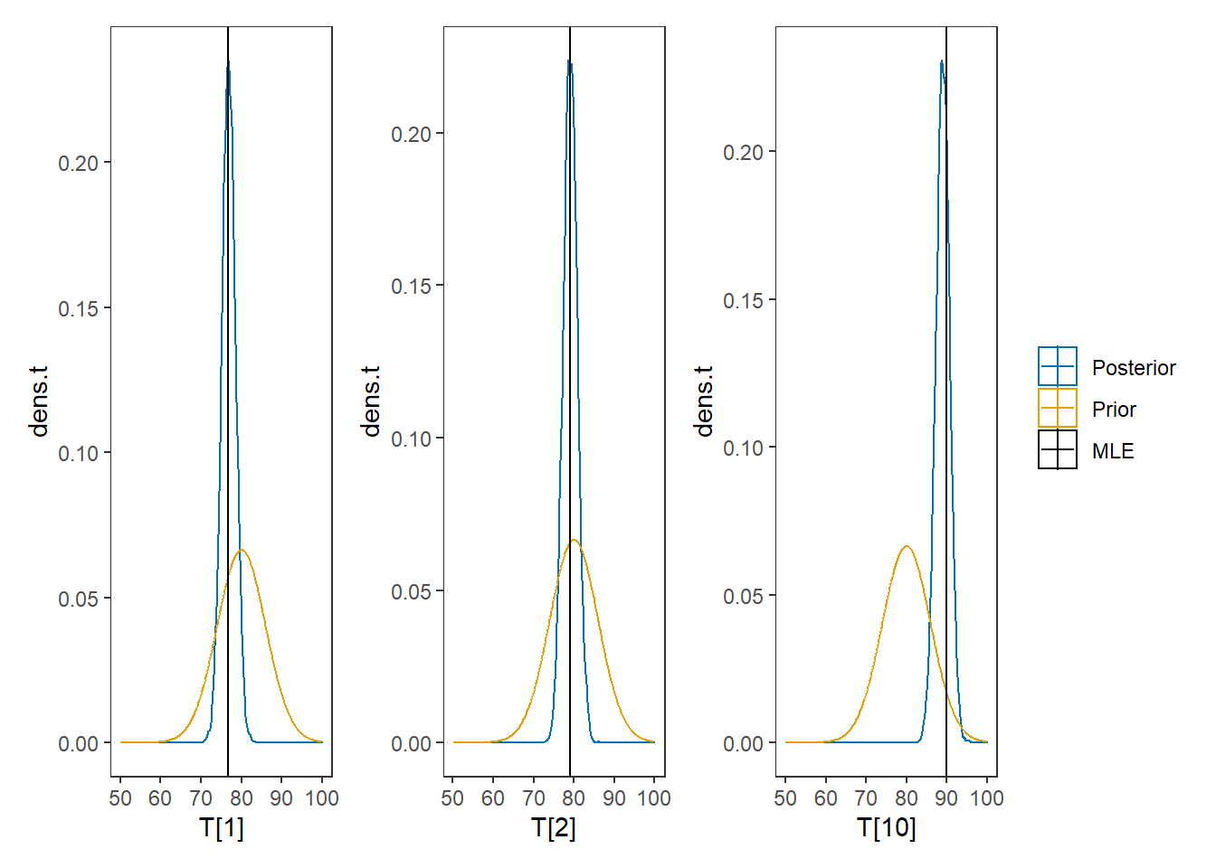
8.7 Example 3 - Unknown Measurement Model with Multiple Measures
Here, we finally get to the (more) realistic case when we don’t have as much prior knowledge about the measurement model parameters (namely, variances). The structure relies on hierarchically specifying priors to induce conditional independence. The DAG and model-specification change to:
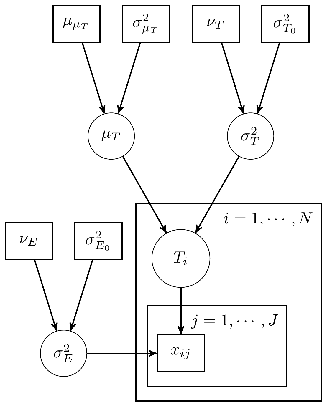
Figure 8.5: Simple CTT model with unknown measurement parameters
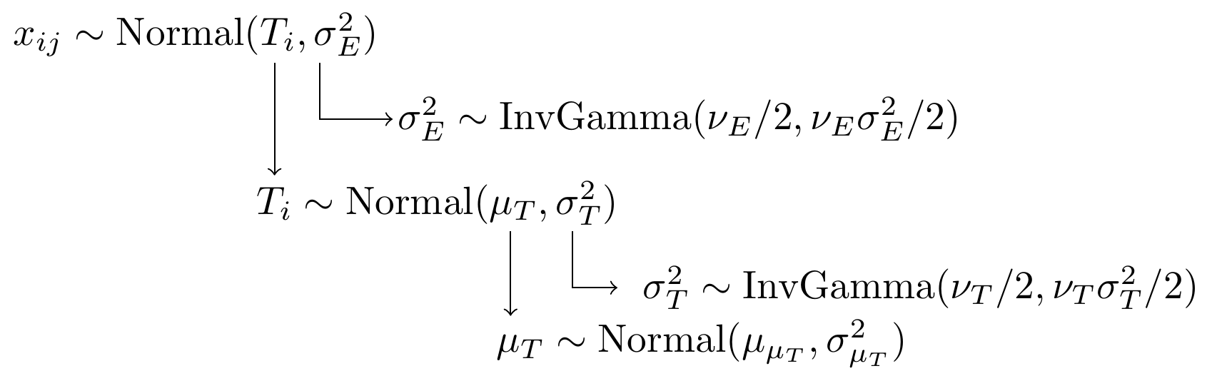
Figure 8.6: Model specification diagram for the unknown measurement model parameters
8.8 Example 3 - Stan
model_ctt3 <- '
data {
  int  N;
  int  J;
  matrix[N, J] X;
}

parameters {
  real T[N];
  real muT;
  real<lower=0> sigmaT;
  real<lower=0> sigmaE;
}

model {
  for(i in 1:N){
    T[i] ~ normal(muT, sigmaT);
    for(j in 1:J){
      X[i, j] ~ normal(T[i], sigmaE);
    }
  }
  muT ~ normal(80, 10);
  sigmaT ~ inv_gamma(1, 6);
  sigmaE ~ inv_gamma(1, 4);
}

generated quantities {
  real rho;
  real rhocomp;

  rho = square(sigmaT)/(square(sigmaT) + square(sigmaE));
  rhocomp = J*rho/((J-1)*rho + 1);
}

'
# data must be in a list
mydata <- list(
  N = 10, J = 5,
  X = matrix(
    c(80, 77, 80, 73, 73,
      83, 79, 78, 78, 77,
      85, 77, 88, 81, 80,
      76, 76, 76, 78, 67,
      70, 69, 73, 71, 77,
      87, 89, 92, 91, 87,
      76, 75, 79, 80, 75,
      86, 75, 80, 80, 82,
      84, 79, 79, 77, 82,
      96, 85, 91, 87, 90),
    ncol=5, nrow=10, byrow=T)
)

# initial values
start_values <- function(){
  list(T=c(80,80,80,80,80,80,80,80,80,80),
       muT=80, sigmaT=10, sigmaE=5)
}

# Next, need to fit the model
#   I have explicitly outlined some common parameters
fit <- stan(
  model_code = model_ctt3, # model code to be compiled
  data = mydata,          # my data
  init = start_values,    # starting values
  chains = 4,             # number of Markov chains
  warmup = 1000,          # number of warm up iterations per chain
  iter = 5000,            # total number of iterations per chain
  cores = 4,              # number of cores (could use one per chain)
  refresh = 0             # no progress shown
)

# first get a basic breakdown of the posteriors
print(fit)
## Inference for Stan model: anon_model.
## 4 chains, each with iter=5000; warmup=1000; thin=1;
## post-warmup draws per chain=4000, total post-warmup draws=16000.
##
## mean se_mean sd 2.5% 25% 50% 75% 97.5% n_eff Rhat
## T[1] 76.86 0.01 1.52 73.90 75.86 76.86 77.86 79.92 24760 1
## T[2] 79.08 0.01 1.52 76.10 78.07 79.08 80.08 82.08 25643 1
## T[3] 82.03 0.01 1.52 79.02 81.01 82.03 83.05 84.97 24831 1
## T[4] 75.02 0.01 1.56 71.98 73.97 75.01 76.08 78.14 23847 1
## T[5] 72.62 0.01 1.56 69.57 71.59 72.60 73.66 75.74 21993 1
## T[6] 88.50 0.01 1.58 85.34 87.48 88.51 89.54 91.57 21711 1
## T[7] 77.23 0.01 1.53 74.22 76.22 77.23 78.26 80.24 22774 1
## T[8] 80.56 0.01 1.52 77.56 79.54 80.55 81.57 83.55 28472 1
## T[9] 80.19 0.01 1.52 77.19 79.19 80.20 81.20 83.17 24704 1
## T[10] 89.05 0.01 1.55 85.88 88.04 89.08 90.09 92.05 21249 1
## muT 80.12 0.01 1.94 76.32 78.88 80.11 81.37 83.91 17196 1
## sigmaT 6.00 0.01 1.63 3.64 4.87 5.72 6.81 10.00 14787 1
## sigmaE 3.50 0.00 0.40 2.82 3.22 3.47 3.75 4.39 15100 1
## rho 0.72 0.00 0.11 0.49 0.65 0.73 0.80 0.90 16035 1
## rhocomp 0.92 0.00 0.04 0.83 0.90 0.93 0.95 0.98 15119 1
## lp__ -115.09 0.04 2.82 -121.51 -116.80 -114.72 -113.03 -110.63 5833 1
##
## Samples were drawn using NUTS(diag_e) at Sun Jun 19 17:35:30 2022.
## For each parameter, n_eff is a crude measure of effective sample size,
## and Rhat is the potential scale reduction factor on split chains (at
## convergence, Rhat=1).
# plot the posterior in a
#  95% probability interval
#  and 80% to contrast the dispersion
plot(fit)
## 'pars' not specified. Showing first 10 parameters by default.## ci_level: 0.8 (80% intervals)## outer_level: 0.95 (95% intervals)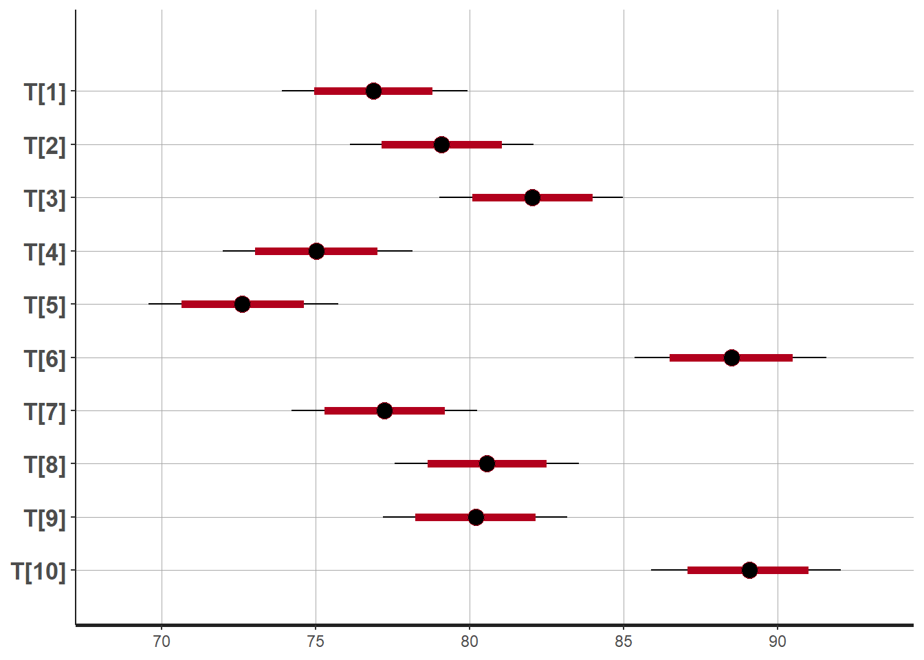
# traceplots
rstan::traceplot(fit, pars = c("T", "muT", "sigmaT", "sigmaE", "rho", "rhocomp"), inc_warmup = TRUE)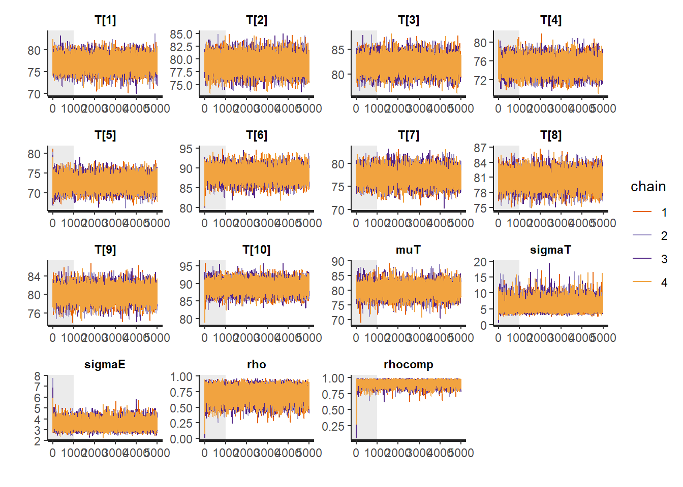
# Gelman-Rubin-Brooks Convergence Criterion
p1 <- ggs_grb(ggs(fit)) +
   theme_bw() + theme(panel.grid = element_blank())
p1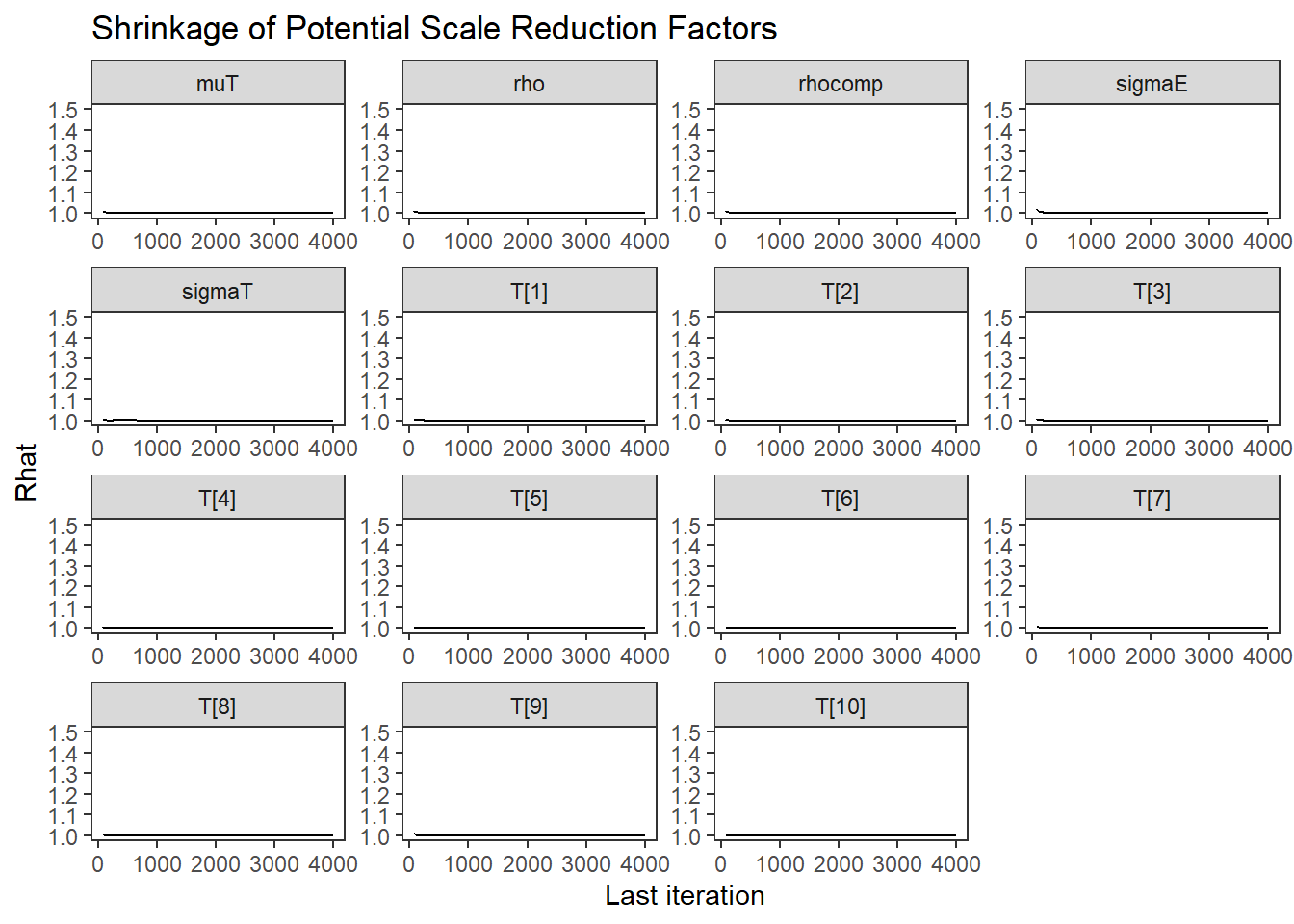
# autocorrelation
p1 <- ggs_autocorrelation(ggs(fit)) +
   theme_bw() + theme(panel.grid = element_blank())
p1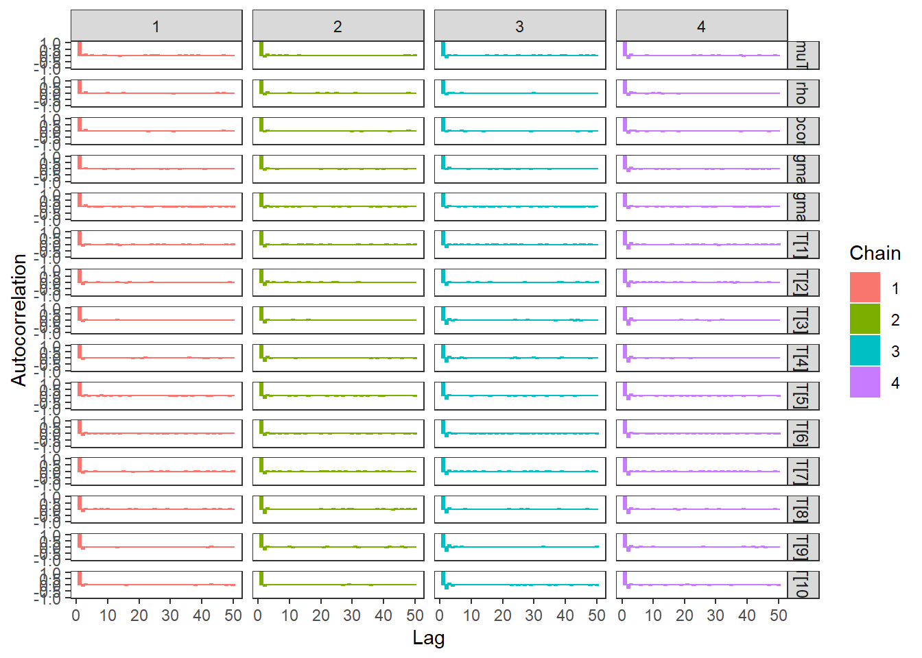
# plot the posterior density
plot.data <- as.matrix(fit)

plot_title <- ggtitle("Posterior distributions",
                      "with medians and 80% intervals")
mcmc_areas(
  plot.data,
  pars = c(paste0("T[",1:10,"]"), "muT"),
  prob = 0.8) +
  plot_title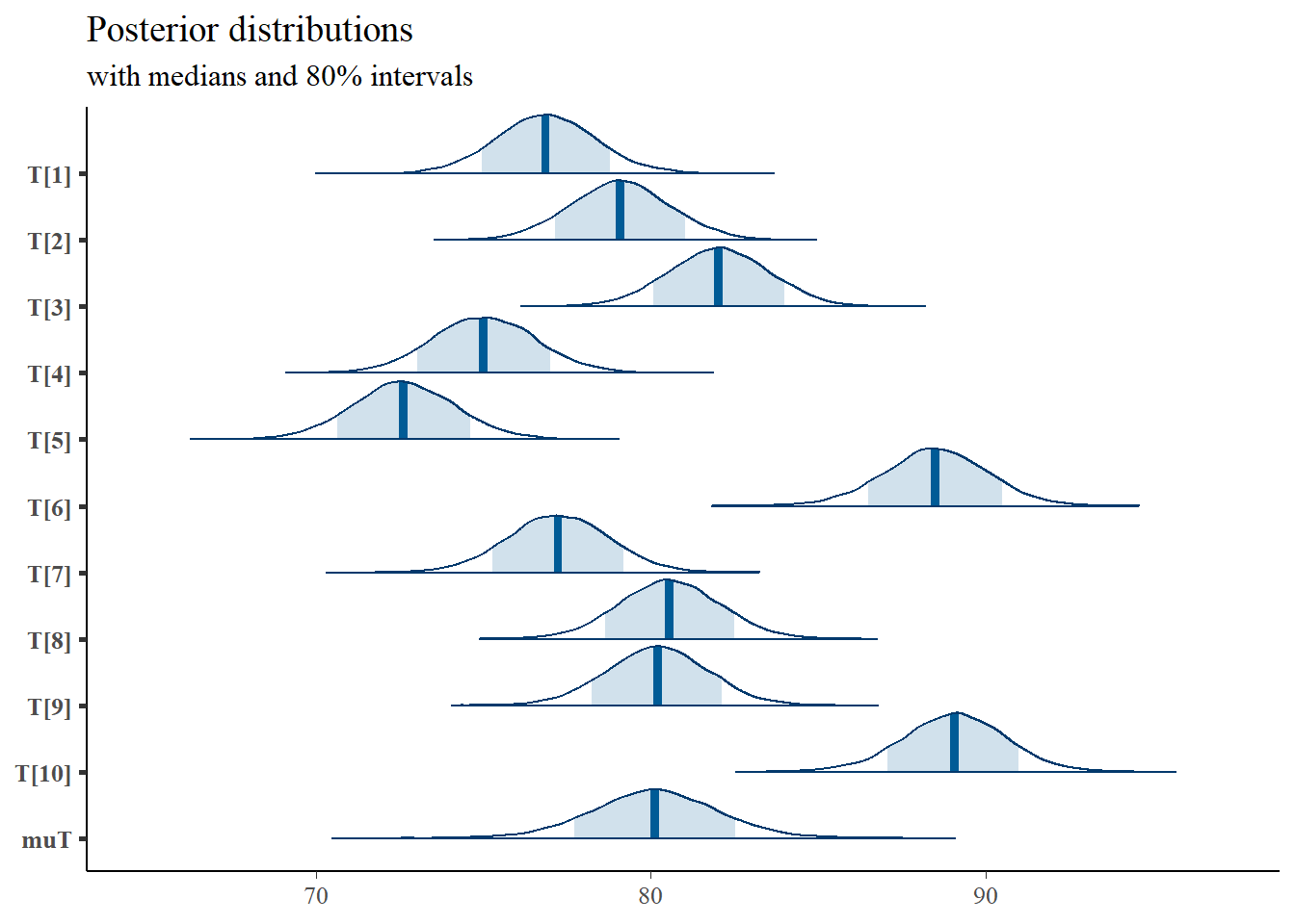
mcmc_areas(
  plot.data,
  pars = c("sigmaT", "sigmaE"),
  prob = 0.8) +
  plot_title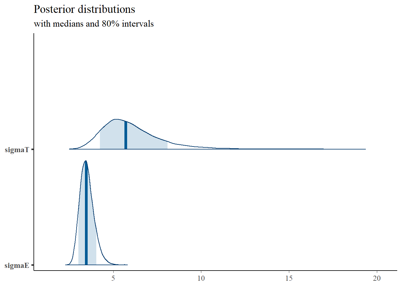
mcmc_areas(
  plot.data,
  pars = c("rho", "rhocomp"),
  prob = 0.8) +
  plot_title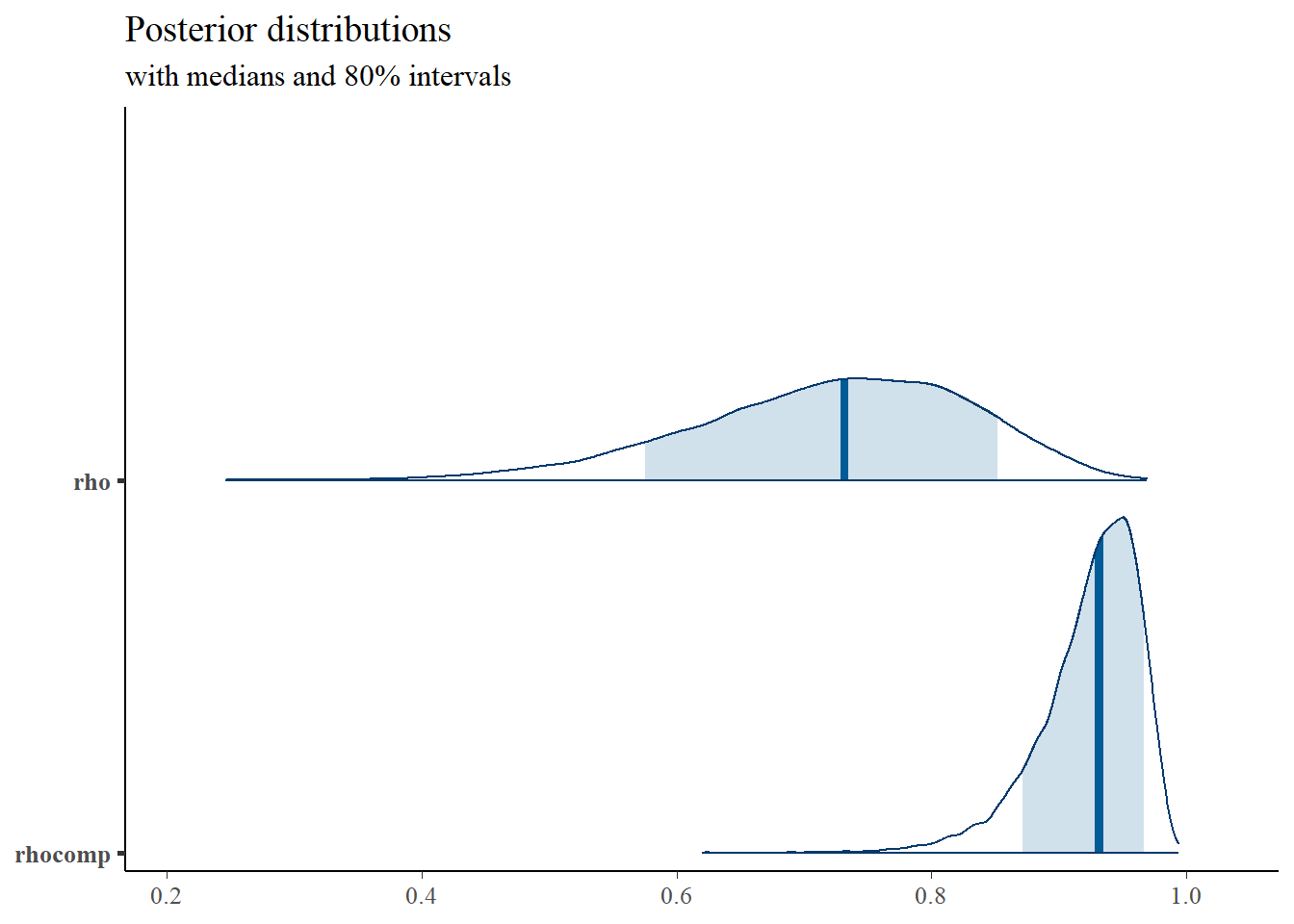
# I prefer a posterior plot that includes prior and MLE
# Expanded Posterior Plot
MLE <- c(rowMeans(mydata$X), mean(mydata$X))

prior_mu <- function(x){dnorm(x, 80, 10)}
x.mu<- seq(50.1, 100, 0.1)
prior.mu <- data.frame(mu=x.mu, dens.mu = prior_mu(x.mu))

prior_sigt <- function(x){dinvgamma(x, 1, 6)}
x.sigt<- seq(.1, 15, 0.1)
prior.sigt <- data.frame(sigt=x.sigt, dens.sigt = prior_sigt(x.sigt))

prior_sige <- function(x){dinvgamma(x, 1, 4)}
x.sige<- seq(.1, 10, 0.1)
prior.sige <- data.frame(sige=x.sige, dens.sige = prior_sige(x.sige))

prior_t <- function(x){
  mu <- rnorm(1, 80, 10)
  sig <- rinvgamma(1, 1, 4)
  rnorm(x, mu, sig)
}
x.t<- seq(50.1, 100, 0.1)
prior.t <- data.frame(tr=prior_t(10000))


cols <- c("Posterior"="#0072B2", "Prior"="#E69F00", "MLE"= "black")#"#56B4E9", "#E69F00" "#CC79A7"
plot.data <- as.data.frame(plot.data)
p1 <- ggplot()+
  geom_density(data=plot.data, aes(x=`T[1]`, color="Posterior"))+
  geom_density(data=prior.t,aes(x=tr,color="Prior"))+
  geom_vline(aes(xintercept=MLE[1], color="MLE"))+
  scale_color_manual(values=cols, name=NULL)+
  theme_bw()+
  theme(panel.grid = element_blank())

p2 <- ggplot()+
  geom_density(data=plot.data, aes(x=`T[5]`, color="Posterior"))+
  geom_density(data=prior.t,aes(x=tr,color="Prior"))+
  geom_vline(aes(xintercept=MLE[5], color="MLE"))+
  scale_color_manual(values=cols, name=NULL)+
  theme_bw()+
  theme(panel.grid = element_blank())

p3 <- ggplot()+
  geom_density(data=plot.data, aes(x=`T[10]`, color="Posterior"))+
  geom_density(data=prior.t,aes(x=tr,color="Prior"))+
  geom_vline(aes(xintercept=MLE[10], color="MLE"))+
  scale_color_manual(values=cols, name=NULL)+
  theme_bw()+
  theme(panel.grid = element_blank())

p4 <- ggplot()+
  geom_density(data=plot.data, aes(x=`muT`, color="Posterior"))+
  geom_line(data=prior.mu,aes(x=mu,y=dens.mu,color="Prior"))+
  geom_vline(aes(xintercept=MLE[11], color="MLE"))+
  scale_color_manual(values=cols, name=NULL)+
  theme_bw()+
  theme(panel.grid = element_blank())

p5 <- ggplot()+
  geom_density(data=plot.data, aes(x=`sigmaT`, color="Posterior"))+
  geom_line(data=prior.sigt,aes(x=sigt,y=dens.sigt,color="Prior"))+
  scale_color_manual(values=cols, name=NULL)+
  theme_bw()+
  theme(panel.grid = element_blank())

p6 <- ggplot()+
  geom_density(data=plot.data, aes(x=`sigmaE`, color="Posterior"))+
  geom_line(data=prior.sige,aes(x=sige,y=dens.sige,color="Prior"))+
  scale_color_manual(values=cols, name=NULL)+
  theme_bw()+
  theme(panel.grid = element_blank())

p1 + p2 + p3 + p4 + p5 + p6 + plot_layout(ncol=3, guides="collect")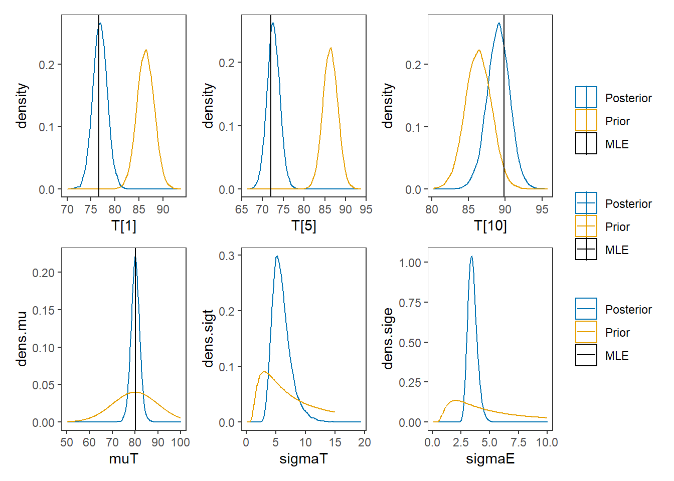
8.9 Example 3 - JAGS
# model code
jags.model.ctt3 <- function(){
     ############################################
     # CLASSICAL TEST THEORY MODEL
     # WITH UnkNOWN HYPERPARAMETERS
     #    TRUE SCORE MEAN, TRUE SCORE VARIANCE
     #    ERROR VARIANCE
     ############################################

     ############################################
     # PRIOR DISTRIBUTIONS FOR HYPERPARAMETERS
     ############################################
     muT ~ dnorm(80,.01)     # Mean of the true scores

     tau.T ~ dgamma(1, 36)   # Precision of the true scores
     tau.E ~ dgamma(1, 16)   # Precision of the errors

     sigma.squared.T <- 1/tau.T    # Variance of the true scores
     sigma.squared.E <- 1/tau.E    # Variance of the errors
     # get SD for summarizing
     sigmaT <- pow(sigma.squared.T, 0.5)
     sigmaE <- pow(sigma.squared.E, 0.5)
     ############################################
     # MODEL FOR TRUE SCORES AND OBSERVABLES
     ############################################

     for (i in 1:N) {
          T[i] ~ dnorm(muT, tau.T)     # Distribution of true scores
          for(j in 1:J){
               X[i,j] ~ dnorm(T[i], tau.E)     # Distribution of observables
          }
     }

     ############################################
     # RELIABILITY
     ############################################
     rho <- sigma.squared.T/(sigma.squared.T+sigma.squared.E)
     rhocomp <- J*rho/((J-1)*rho+1)

}
# data
mydata <- list(
  N = 10, J = 5,
  X = matrix(
    c(80, 77, 80, 73, 73,
      83, 79, 78, 78, 77,
      85, 77, 88, 81, 80,
      76, 76, 76, 78, 67,
      70, 69, 73, 71, 77,
      87, 89, 92, 91, 87,
      76, 75, 79, 80, 75,
      86, 75, 80, 80, 82,
      84, 79, 79, 77, 82,
      96, 85, 91, 87, 90),
    ncol=5, nrow=10, byrow=T)
)

# initial values
start_values <- list(
  list("T"=c(60,85,80,95,74,69,91,82,87,78),
       "muT"=80, "tau.E"=0.06, "tau.T"=0.023),
  list("T"=c(63, 79, 74, 104, 80, 71, 95, 72, 80, 82),
       "muT"=100, "tau.E"=0.09, "tau.T"=0.05),
  list("T"=c(59, 86, 88, 89, 76, 65, 94, 72, 95, 84),
       "muT"=70, "tau.E"=0.03, "tau.T"=0.001),
  list("T"=c(60, 87, 90, 91, 77, 74, 95, 76, 83, 87),
       "muT"=90, "tau.E"=0.01, "tau.T"=0.1)
)

# vector of all parameters to save
param_save <- c("T","muT","sigmaT","sigmaE", "rho", "rhocomp")

# fit model
fit <- jags(
  model.file=jags.model.ctt2,
  data=mydata,
  inits=start_values,
  parameters.to.save = param_save,
  n.iter=4000,
  n.burnin = 1000,
  n.chains = 4,
  n.thin=1,
  progress.bar = "none")
## Warning in jags.model(model.file, data = data, inits = init.values, n.chains = n.chains, : Unused
## variable "X" in data## Compiling model graph
## Resolving undeclared variables
## Allocating nodes
## Graph information:
## Observed stochastic nodes: 0
## Unobserved stochastic nodes: 60
## Total graph size: 68
##
## Deleting model## Error in setParameters(init.values[[i]], i): Error in node tau.E
## Cannot set value of non-variable node
print(fit)## Inference for Stan model: anon_model.
## 4 chains, each with iter=5000; warmup=1000; thin=1;
## post-warmup draws per chain=4000, total post-warmup draws=16000.
##
## mean se_mean sd 2.5% 25% 50% 75% 97.5% n_eff Rhat
## T[1] 76.86 0.01 1.52 73.90 75.86 76.86 77.86 79.92 24760 1
## T[2] 79.08 0.01 1.52 76.10 78.07 79.08 80.08 82.08 25643 1
## T[3] 82.03 0.01 1.52 79.02 81.01 82.03 83.05 84.97 24831 1
## T[4] 75.02 0.01 1.56 71.98 73.97 75.01 76.08 78.14 23847 1
## T[5] 72.62 0.01 1.56 69.57 71.59 72.60 73.66 75.74 21993 1
## T[6] 88.50 0.01 1.58 85.34 87.48 88.51 89.54 91.57 21711 1
## T[7] 77.23 0.01 1.53 74.22 76.22 77.23 78.26 80.24 22774 1
## T[8] 80.56 0.01 1.52 77.56 79.54 80.55 81.57 83.55 28472 1
## T[9] 80.19 0.01 1.52 77.19 79.19 80.20 81.20 83.17 24704 1
## T[10] 89.05 0.01 1.55 85.88 88.04 89.08 90.09 92.05 21249 1
## muT 80.12 0.01 1.94 76.32 78.88 80.11 81.37 83.91 17196 1
## sigmaT 6.00 0.01 1.63 3.64 4.87 5.72 6.81 10.00 14787 1
## sigmaE 3.50 0.00 0.40 2.82 3.22 3.47 3.75 4.39 15100 1
## rho 0.72 0.00 0.11 0.49 0.65 0.73 0.80 0.90 16035 1
## rhocomp 0.92 0.00 0.04 0.83 0.90 0.93 0.95 0.98 15119 1
## lp__ -115.09 0.04 2.82 -121.51 -116.80 -114.72 -113.03 -110.63 5833 1
##
## Samples were drawn using NUTS(diag_e) at Sun Jun 19 17:35:30 2022.
## For each parameter, n_eff is a crude measure of effective sample size,
## and Rhat is the potential scale reduction factor on split chains (at
## convergence, Rhat=1).
# extract posteriors for all chains
jags.mcmc <- as.mcmc(fit)

R2jags::traceplot(jags.mcmc)
## Error in xy.coords(x, y, xlabel, ylabel, log = log, recycle = TRUE): 'list' object cannot be coerced to type 'double'
# gelman-rubin-brook
gelman.plot(jags.mcmc)
## Error in gelman.preplot(x, bin.width = bin.width, max.bins = max.bins, : Insufficient iterations to produce Gelman-Rubin plot
# convert to single data.frame for density plot
a <- colnames(as.data.frame(jags.mcmc[[1]]))
## Error in jags.mcmc[[1]]: this S4 class is not subsettable
plot.data <- data.frame(as.matrix(jags.mcmc, chains=T, iters = T))## Error in y[, var.cols] <- x: number of items to replace is not a multiple of replacement length
colnames(plot.data) <- c("chain", "iter", a)


plot_title <- ggtitle("Posterior distributions",
                      "with medians and 80% intervals")
mcmc_areas(
  plot.data,
  pars = c(paste0("T[",1:10,"]"), "muT"),
  prob = 0.8) +
  plot_title
## Error in x[, j, ] <- a[chain == j, , drop = FALSE]: replacement has length zero
mcmc_areas(
  plot.data,
  pars = c("sigmaT", "sigmaE"),
  prob = 0.8) +
  plot_title
## Error in x[, j, ] <- a[chain == j, , drop = FALSE]: replacement has length zero
mcmc_areas(
  plot.data,
  pars = c("rho", "rhocomp"),
  prob = 0.8) +
  plot_title
## Error in x[, j, ] <- a[chain == j, , drop = FALSE]: replacement has length zero
# I prefer a posterior plot that includes prior and MLE
MLE <- c(rowMeans(mydata$X), mean(mydata$X))

prior_mu <- function(x){dnorm(x, 80, 10)}
x.mu<- seq(50.1, 100, 0.1)
prior.mu <- data.frame(mu=x.mu, dens.mu = prior_mu(x.mu))

prior_sigt <- function(x){dinvgamma(x, 1, 6)}
x.sigt<- seq(.1, 15, 0.1)
prior.sigt <- data.frame(sigt=x.sigt, dens.sigt = prior_sigt(x.sigt))

prior_sige <- function(x){dinvgamma(x, 1, 4)}
x.sige<- seq(.1, 10, 0.1)
prior.sige <- data.frame(sige=x.sige, dens.sige = prior_sige(x.sige))

prior_t <- function(x){
  mu <- rnorm(1, 80, 10)
  sig <- rinvgamma(1, 1, 4)
  rnorm(x, mu, sig)
}
x.t<- seq(50.1, 100, 0.1)
prior.t <- data.frame(tr=prior_t(10000))
cols <- c("Posterior"="#0072B2", "Prior"="#E69F00", "MLE"= "black")#"#56B4E9", "#E69F00" "#CC79A7"

p1 <- ggplot()+
  geom_density(data=plot.data, aes(x=`T[1]`, color="Posterior"))+
  geom_density(data=prior.t,aes(x=tr,color="Prior"))+
  geom_vline(aes(xintercept=MLE[1], color="MLE"))+
  scale_color_manual(values=cols, name=NULL)+
  theme_bw()+
  theme(panel.grid = element_blank())

p2 <- ggplot()+
  geom_density(data=plot.data, aes(x=`T[5]`, color="Posterior"))+
  geom_density(data=prior.t,aes(x=tr,color="Prior"))+
  geom_vline(aes(xintercept=MLE[5], color="MLE"))+
  scale_color_manual(values=cols, name=NULL)+
  theme_bw()+
  theme(panel.grid = element_blank())

p3 <- ggplot()+
  geom_density(data=plot.data, aes(x=`T[10]`, color="Posterior"))+
  geom_density(data=prior.t,aes(x=tr,color="Prior"))+
  geom_vline(aes(xintercept=MLE[10], color="MLE"))+
  scale_color_manual(values=cols, name=NULL)+
  theme_bw()+
  theme(panel.grid = element_blank())

p4 <- ggplot()+
  geom_density(data=plot.data, aes(x=`muT`, color="Posterior"))+
  geom_line(data=prior.mu,aes(x=mu,y=dens.mu,color="Prior"))+
  geom_vline(aes(xintercept=MLE[11], color="MLE"))+
  scale_color_manual(values=cols, name=NULL)+
  theme_bw()+
  theme(panel.grid = element_blank())

p5 <- ggplot()+
  geom_density(data=plot.data, aes(x=`sigmaT`, color="Posterior"))+
  geom_line(data=prior.sigt,aes(x=sigt,y=dens.sigt,color="Prior"))+
  scale_color_manual(values=cols, name=NULL)+
  theme_bw()+
  theme(panel.grid = element_blank())

p6 <- ggplot()+
  geom_density(data=plot.data, aes(x=`sigmaE`, color="Posterior"))+
  geom_line(data=prior.sige,aes(x=sige,y=dens.sige,color="Prior"))+
  scale_color_manual(values=cols, name=NULL)+
  theme_bw()+
  theme(panel.grid = element_blank())

p1 + p2 + p3 + p4 + p5 + p6 + plot_layout(ncol=3, guides="collect")
## Error in FUN(X[[i]], ...): object 'muT' not found