9 Confirmatory Factor Analysis
The full Bayesian specification of a general CFA model for all associated unknowns is as follows. This includes probability statements, notation, parameters, likelihood, priors, and hyperparameters. The observed data is defined as the \(n\times J\) matrix \(\mathbf{X}\) for the \(J\) observed measures. The CFA model parameters are defined as
\[\begin{align*} \mathbf{x}_i &= \tau + \Lambda\xi_i + \varepsilon_i\\ \Sigma (\mathbf{x}) &= \Lambda\Phi\Lambda^{\prime} + \Psi \end{align*}\]
- \(\Xi\) is the \(n\times M\) matrix of latent variable scores on the \(M\) latent variables for the \(n\) respondents/subjects. For an single subject, \(\xi_i\) represents the vector of scores on the latent variable(s). Values (location, scale, orientation, etc.) or \(\xi_i\) are conditional on (1) \(\kappa\), the \(M\times 1\) vector of latent variable means, and (2) \(\Phi\), the \(M\times M\) covariance matrix of variable variables;
- \(\tau\) is the \(J\times 1\) vector of observed variable intercepts which is the expected value for the observed measures when the latent variable(s) are all \(0\);
- \(\Lambda\) is the \(J\times M\) matrix of factor loadings where the \(j\)th row and \(m\)th column represents the factor loading of the \(j\)th observed variable on the \(m\)th latent variable;
- \(\delta_i\) is the \(J\times 1\) vector of errors, where \(E(\delta_i)=\mathbf{0}\) with \(\mathrm{var}(\delta_i)=\Psi\) which is the \(J\times J\) error covariance matrix.
\[\begin{align*} p(\Xi, \kappa, \Phi, \tau, \Lambda, \Psi\mid \mathbf{X}) &\propto p(\mathbf{X}\mid\Xi, \kappa, \Phi, \tau, \Lambda, \Psi)p(\Xi, \kappa, \Phi, \tau, \Lambda, \Psi)\\ &= p(\mathbf{X}\mid\Xi, \kappa, \Phi, \tau, \Lambda, \Psi) p(\Xi\mid\kappa, \Phi) p(\kappa) p(\Phi) p(\tau) p(\Lambda) p(\Psi)\\ &= \prod_{i=1}^{n}\prod_{j=1}^J\prod_{m=1}^M p(x_{ij}\mid\xi_i, \tau_j,\lambda_j, \psi_{jj}) p(\xi_i\mid\kappa, \Phi) p(\kappa_m) p(\Phi) p(\tau_j) p(\lambda_j) p(\psi_{jj}) \end{align*}\] where
\[\begin{align*} x_{ij}\mid\xi_i, \tau_j,\lambda_j, \psi_{jj} &\sim \mathrm{Normal}(\tau_j+\xi_i\lambda^{\prime}_j, \psi_{jj}),\ \mathrm{for}\ i=1, \cdots, n,\ j = 1, \cdots, J;\\ \xi_i\mid\kappa, \Phi &\sim \mathrm{Normal}(\kappa, \Phi),\ \mathrm{for}\ i=1, \cdots, n;\\ \kappa_m &\sim \mathrm{Normal}(\mu_{\kappa},\sigma^2_{\kappa}),\ \mathrm{for}\ m = 1, \cdots, M;\\ \Phi &\sim \mathrm{Inverse-Wishart}(\Phi_0, d);\\ \tau_j &\sim \mathrm{Normal}(\mu_{\tau},\sigma^2_{\tau}),\ \mathrm{for}\ j = 1, \cdots, J;\\ \lambda_{j,m} &\sim \mathrm{Normal}(\mu_{\lambda}, \sigma^2_{\lambda}),\ \mathrm{for}\ j = 1, \cdots, J,\ m = 1, \cdots, M;\\ \psi_{jj} &\sim \mathrm{Inverse-Gamma}(\nu_{\psi}/2, \nu_{\psi}\psi_0/2),\ \mathrm{for}\ j=1, \cdots, J. \end{align*}\] With the hyperparameters that are supplied by the analyst being defined as
- \(\mu_{\kappa}\) is the prior mean for the latent variable,
- \(\sigma^2_{\kappa}\) is the prior variance for the latent variable,
- \(\Phi_0\) is the prior expectation for the covariance matrix among latent variables,
- \(d\) represents a dispersion parameter reflecting the magnitude of our beliefs about \(\Phi_0\),
- \(\mu_{\tau}\) is the prior mean for the intercepts which reflects our knowledge about the location of the observed variables,
- \(\sigma^2_{\tau}\) is a measure of how much weight we want to give to the prior mean,
- \(\mu_{\lambda}\) is the prior mean for the factor loadings which can vary over items and latent variables,
- \(\sigma^2_{\lambda}\) is the measure of dispersion for the the factor loadings, where lower variances indicate a stronger belief about the values for the loadings,
- \(\nu_{\psi}\) is the measure of location for the gamma prior indicating our expectation for the magnitude of the error variance,
- \(\psi_0\) is our uncertainty with respect to the location we selected for the variance, and
- Alternatively, we could place a prior on \(\Psi\) instead of the individual residual variances. This would mean we would be placing a prior on the error-covariance matrix similar to how we specified a prior for latent variance covariance matrix.
9.1 Single Latent Variable Model
Here we consider the model in section 9.3 which is a CFA model with 1 latent variable and 5 observed indicators. The graphical representation of these factor models get pretty complex pretty quickly, but for this example I have reproduced a version of Figure 9.3b, shown below.
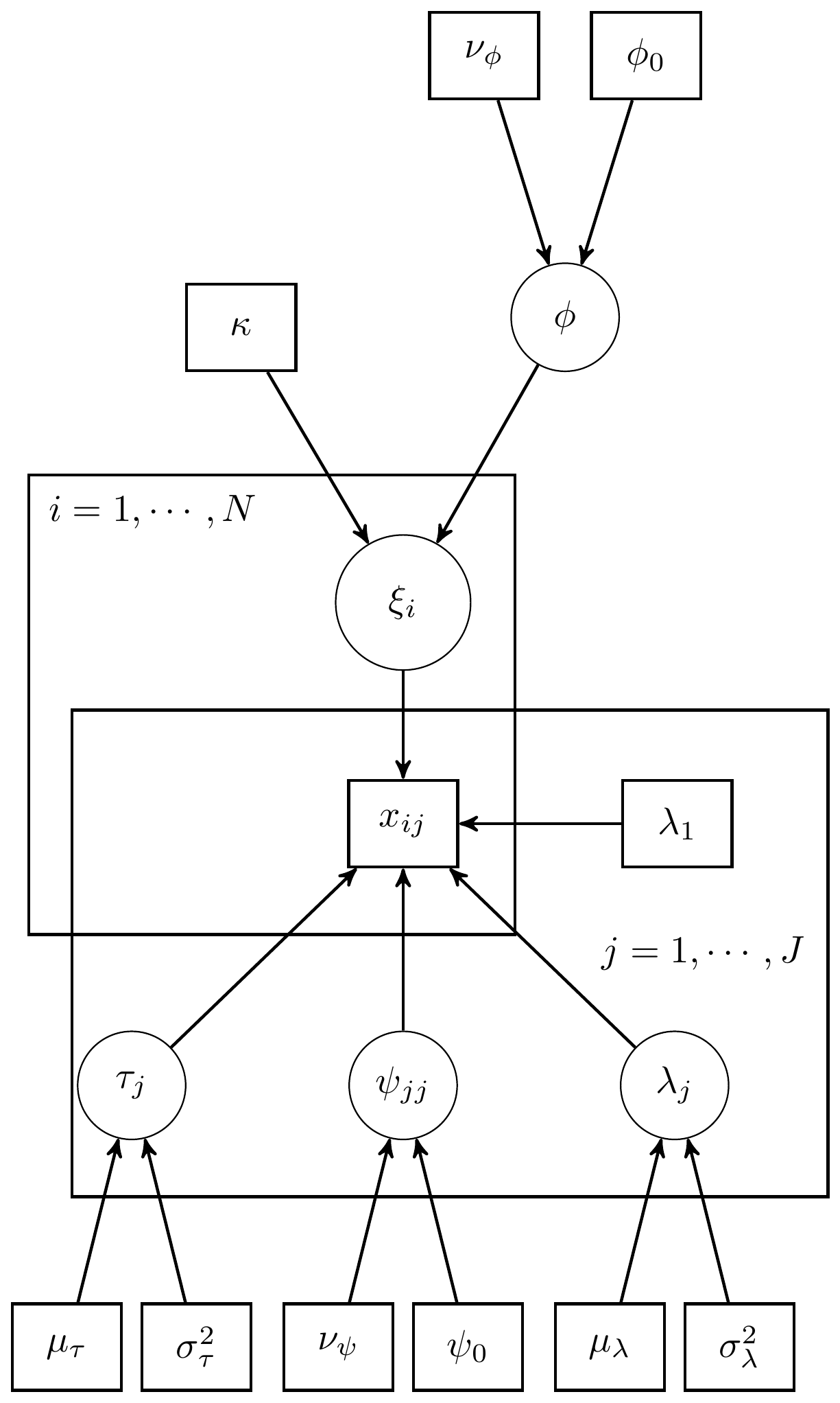
Figure 9.1: DAG for CFA model with 1 latent variable
However, as the authors noted, the path diagram tradition of conveying models is also very useful in discussing and describing the model, which I give next.
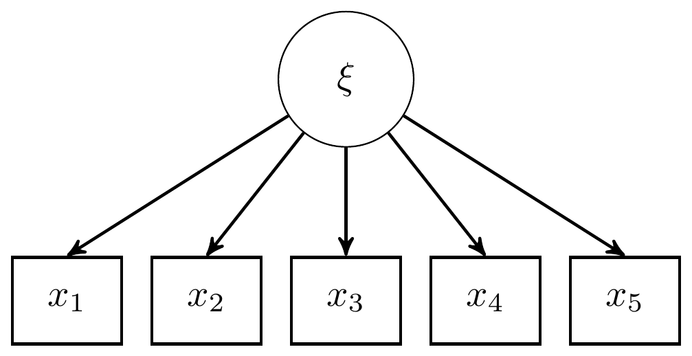
Figure 9.2: Path diagram for CFA model with 1 latent variable
For completeness, I have included the model specification diagram that more concretely connects the DAG and path diagram to the assumed distributions and priors.
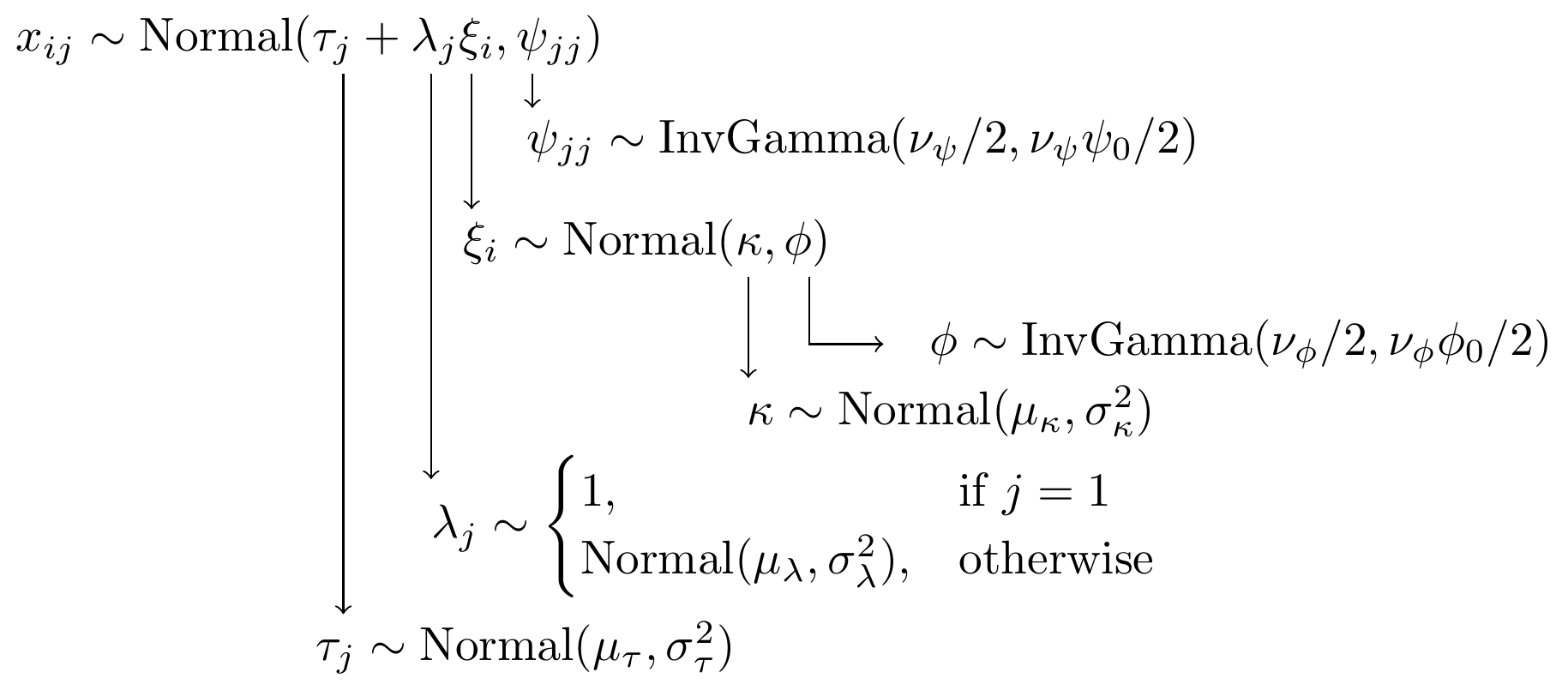
Figure 9.3: Model specification diagram for the CFA model with 1 latent factor
9.2 JAGS - Single Latent Variable
# model code
jags.model.cfa1 <- function(){

  ########################################
  # Specify the factor analysis measurement model for the observables
  ##############################################
  for (i in 1:n){
    for(j in 1:J){
      mu[i,j] <- tau[j] + ksi[i]*lambda[j]      # model implied expectation for each observable
      x[i,j] ~ dnorm(mu[i,j], inv.psi[j])    # distribution for each observable
    }
  }


  ##################################
  # Specify the (prior) distribution for the latent variables
  ####################################
  for (i in 1:n){
    ksi[i] ~ dnorm(kappa, inv.phi)  # distribution for the latent variables
  }


  ######################################
  # Specify the prior distribution for the parameters that govern the latent variables
  ###################################
  kappa <- 0              # Mean of factor 1
  inv.phi ~ dgamma(5, 10) # Precision of factor 1
  phi <- 1/inv.phi        # Variance of factor 1


  ########################################
  # Specify the prior distribution for the measurement model parameters
  ########################################
  for(j in 1:J){
    tau[j] ~ dnorm(3, .1)        # Intercepts for observables
    inv.psi[j] ~ dgamma(5, 10) # Precisions for observables
    psi[j] <- 1/inv.psi[j]   # Variances for observables
  }

  lambda[1] <- 1.0              # loading fixed to 1.0
  for (j in 2:J){
    lambda[j] ~ dnorm(1, .1)    # prior distribution for the remaining loadings
  }
}
# data must be in a list
dat <- read.table("code/CFA-One-Latent-Variable/Data/IIS.dat", header=T)

mydata <- list(
  n = 500, J = 5,
  x = as.matrix(dat)
)


# initial values
start_values <- list(
  list("tau"=c(.1, .1, .1, .1, .1),
       "lambda"=c(NA, 0, 0, 0, 0),
       "inv.phi"=1,
       "inv.psi"=c(1, 1, 1, 1, 1)),
  list("tau"=c(3, 3, 3, 3, 3),
       "lambda"=c(NA, 3, 3, 3, 3),
       "inv.phi"=2,
       "inv.psi"=c(2, 2, 2, 2, 2)),
  list("tau"=c(5, 5, 5, 5, 5),
       "lambda"=c(NA, 6, 6, 6, 6),
       "inv.phi"=.5,
       "inv.psi"=c(.5, .5, .5, .5, .5))
)

# vector of all parameters to save
# exclude fixed lambda since it throws an error in
# in the GRB plot
param_save <- c("tau", paste0("lambda[",2:5,"]"), "phi", "psi")

# fit model
fit <- jags(
  model.file=jags.model.cfa1,
  data=mydata,
  inits=start_values,
  parameters.to.save = param_save,
  n.iter=5000,
  n.burnin = 2500,
  n.chains = 3,
  n.thin=1,
  progress.bar = "none")
## module glm loaded## Compiling model graph
## Resolving undeclared variables
## Allocating nodes
## Graph information:
## Observed stochastic nodes: 2500
## Unobserved stochastic nodes: 515
## Total graph size: 8029
##
## Initializing model
print(fit)## Inference for Bugs model at "C:/Users/noahp/AppData/Local/Temp/RtmpaGlb2m/model324459da2493.txt", fit using jags,
## 3 chains, each with 5000 iterations (first 2500 discarded)
## n.sims = 7500 iterations saved
## mu.vect sd.vect 2.5% 25% 50% 75% 97.5% Rhat n.eff
## lambda[2] 0.730 0.045 0.646 0.699 0.729 0.760 0.820 1.001 7500
## lambda[3] 0.421 0.037 0.351 0.396 0.420 0.445 0.495 1.001 7500
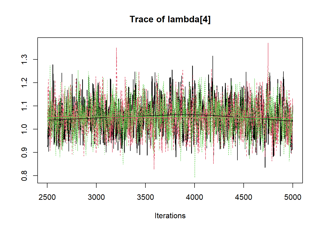
## lambda[4] 1.053 0.066 0.930 1.008 1.051 1.095 1.187 1.001 6000
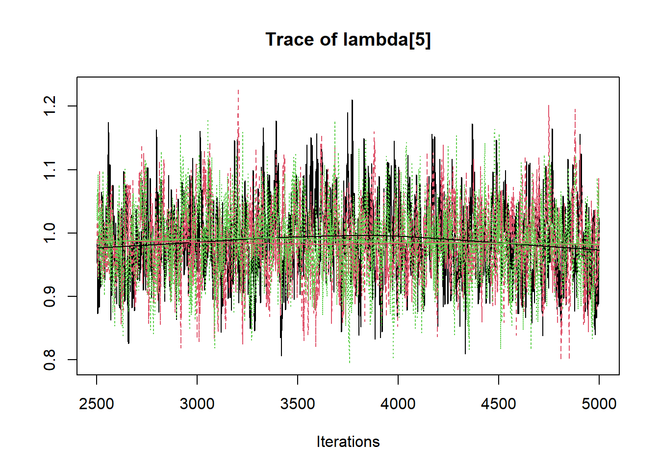
## lambda[5] 0.987 0.059 0.875 0.947 0.985 1.026 1.107 1.002 2400
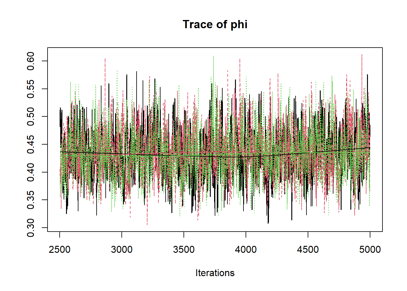
## phi 0.434 0.043 0.354 0.404 0.432 0.463 0.524 1.002 2600
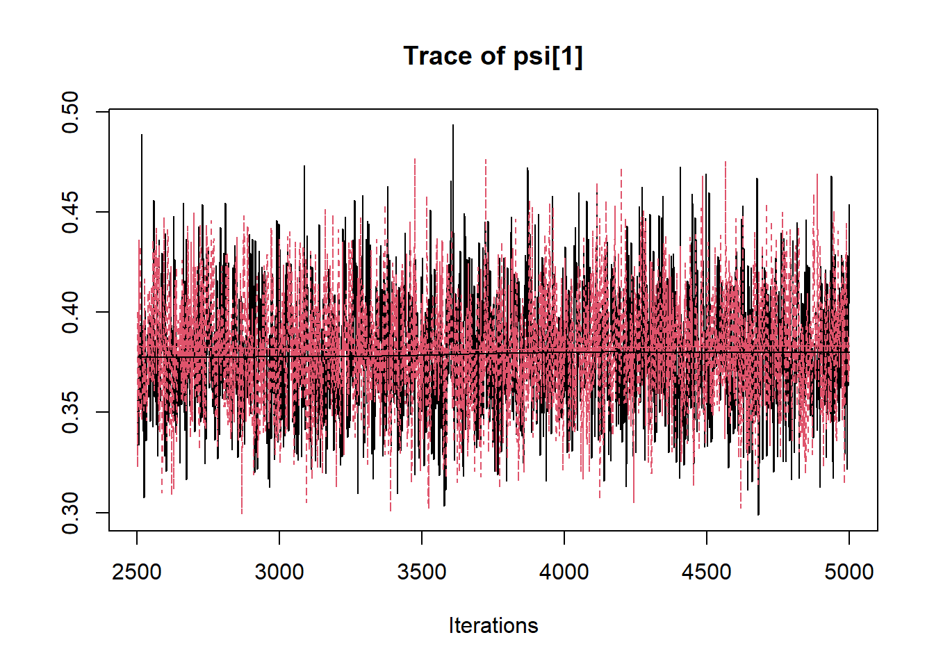
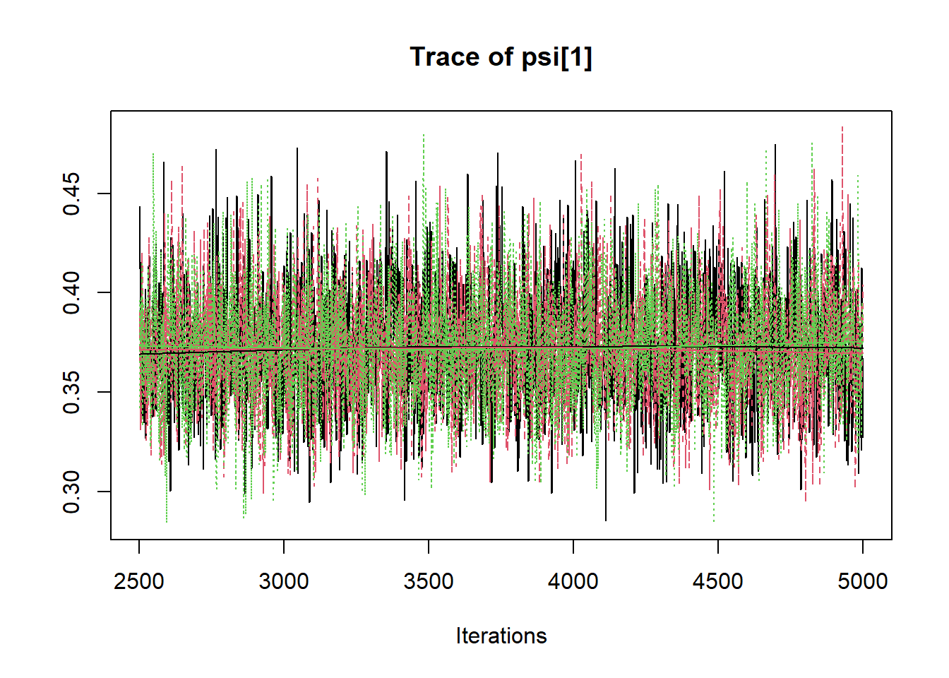
## psi[1] 0.373 0.028 0.320 0.353 0.372 0.391 0.433 1.001 7500
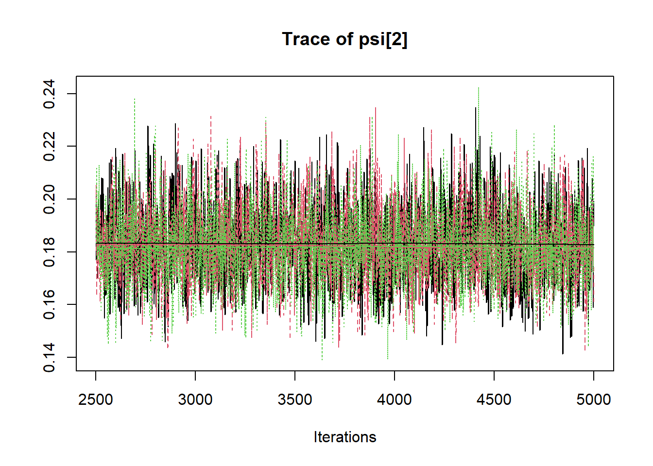
## psi[2] 0.183 0.014 0.157 0.173 0.182 0.192 0.212 1.003 1100
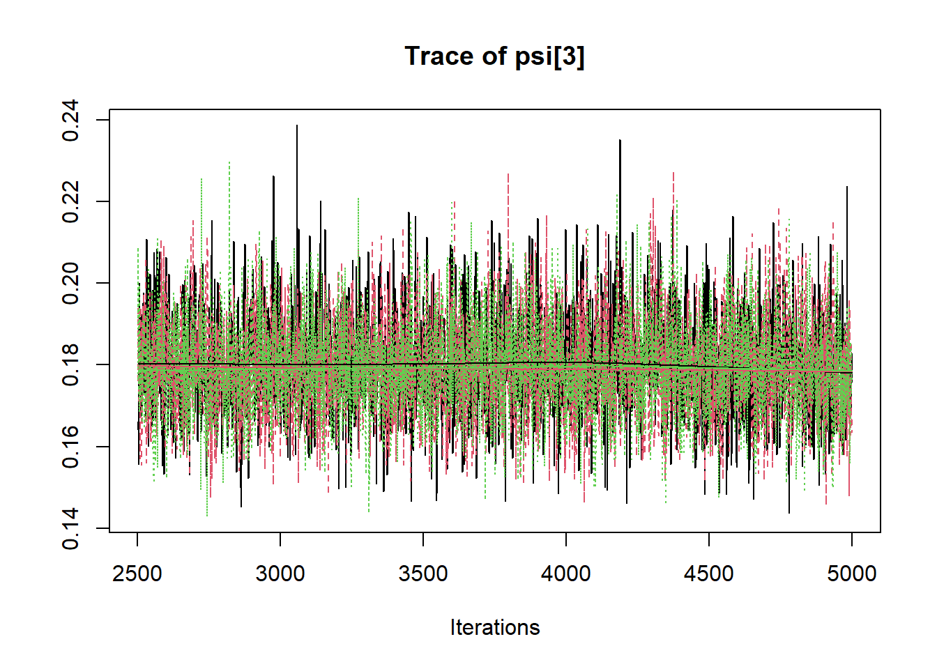
## psi[3] 0.180 0.012 0.157 0.171 0.179 0.187 0.205 1.002 1400
## psi[4] 0.378 0.030 0.323 0.357 0.376 0.398 0.440 1.001 3800
## psi[5] 0.265 0.022 0.225 0.250 0.264 0.279 0.309 1.002 2500
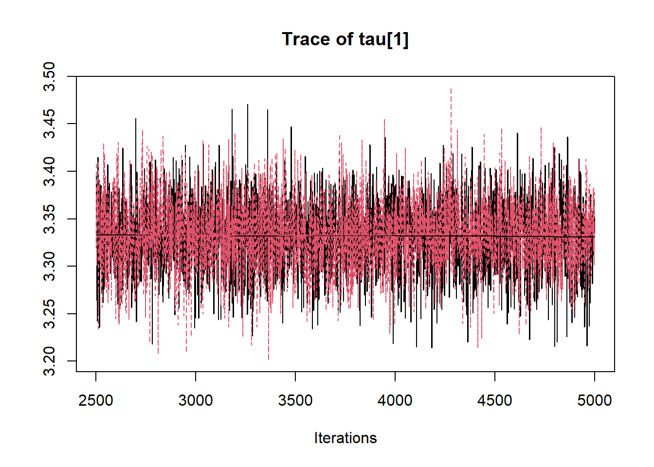
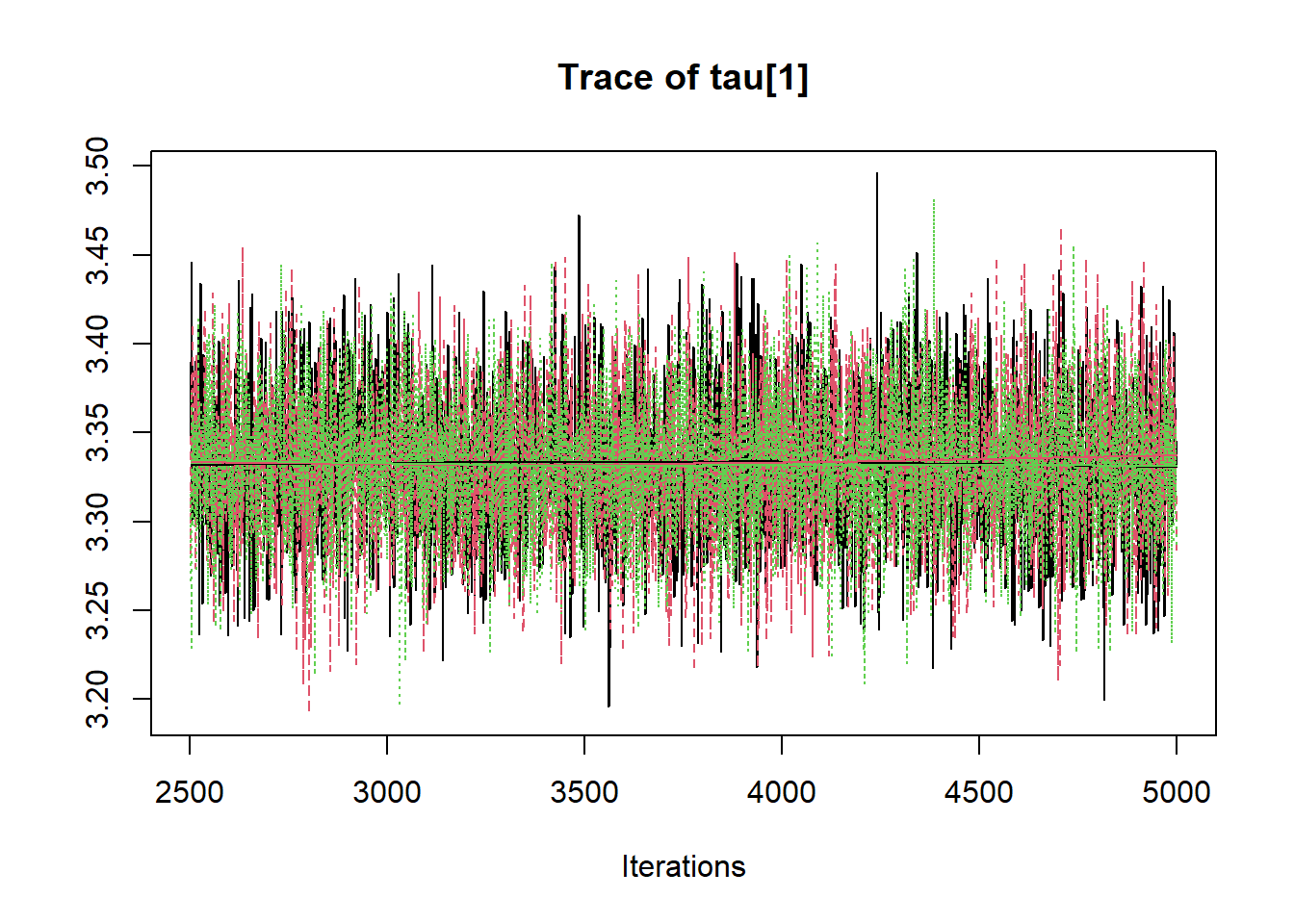
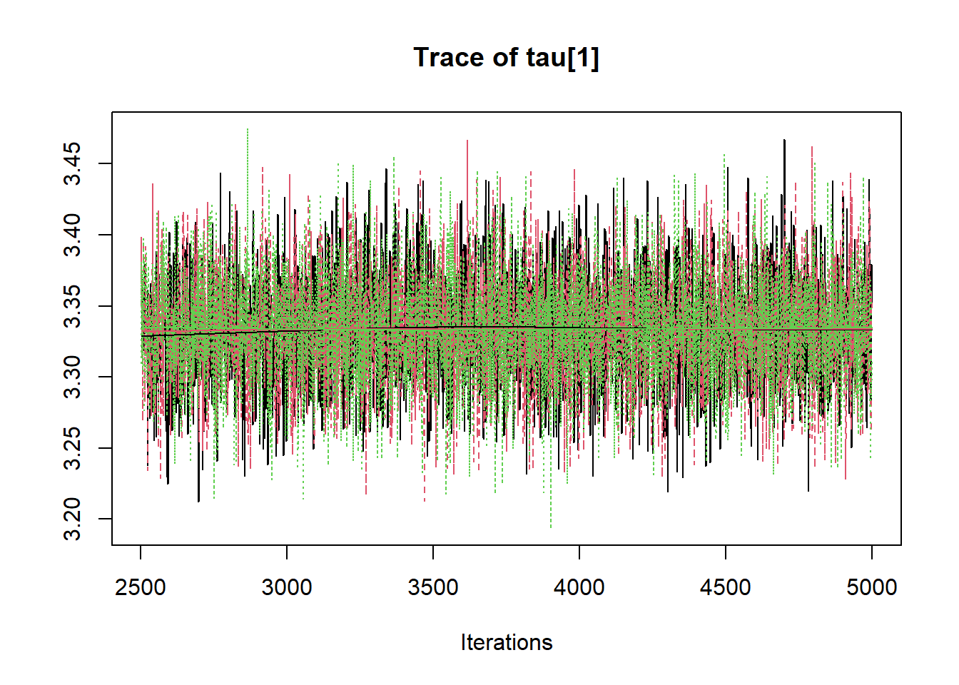
## tau[1] 3.333 0.040 3.255 3.305 3.333 3.359 3.412 1.001 7500
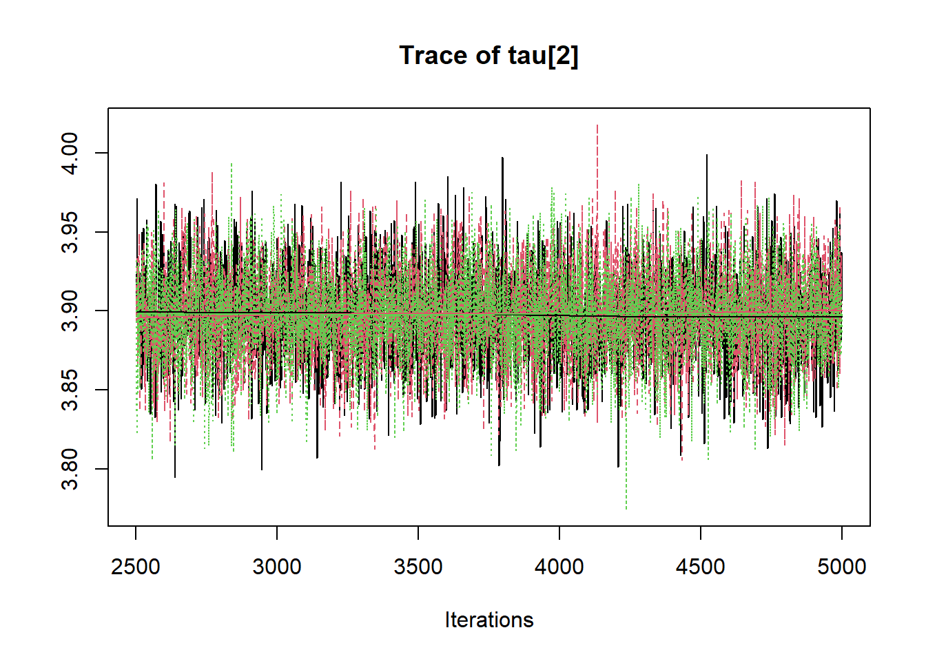
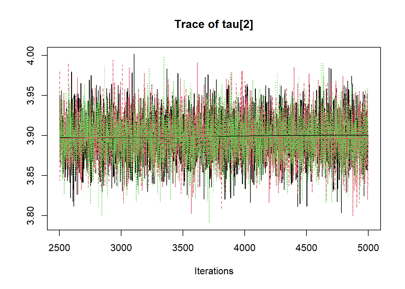
## tau[2] 3.898 0.029 3.841 3.879 3.898 3.917 3.955 1.001 7500
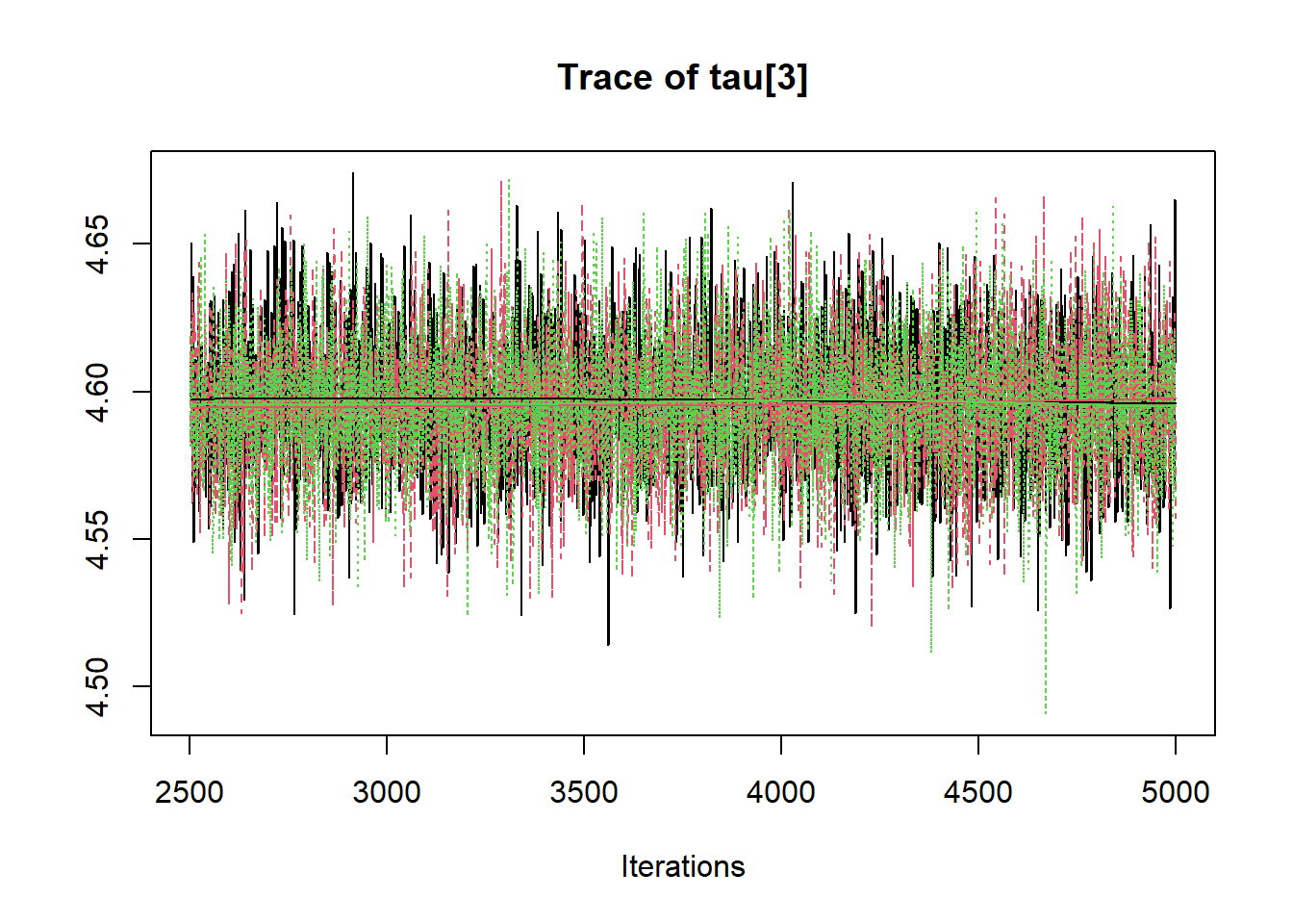
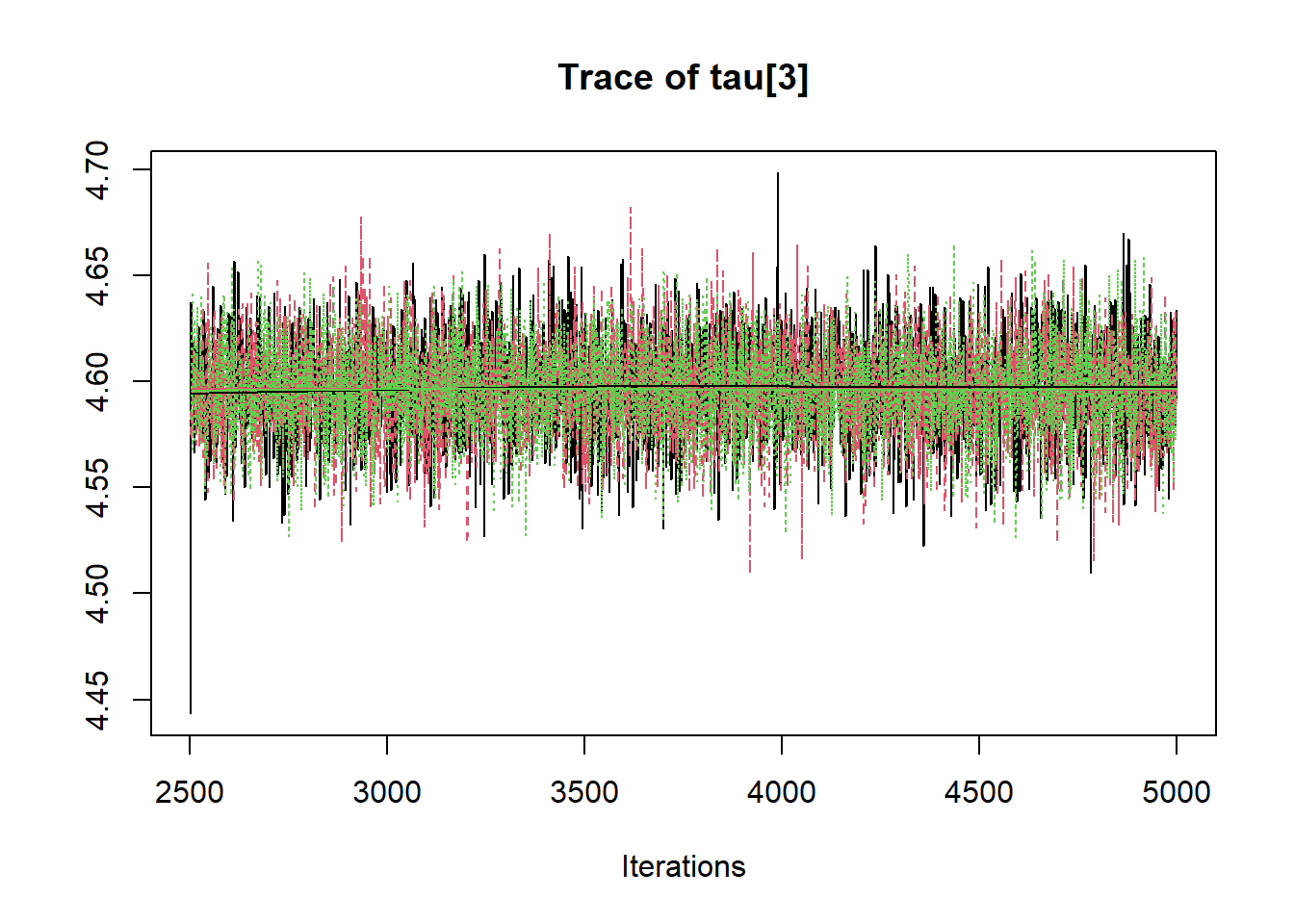
## tau[3] 4.596 0.023 4.553 4.581 4.596 4.611 4.641 1.002 2300
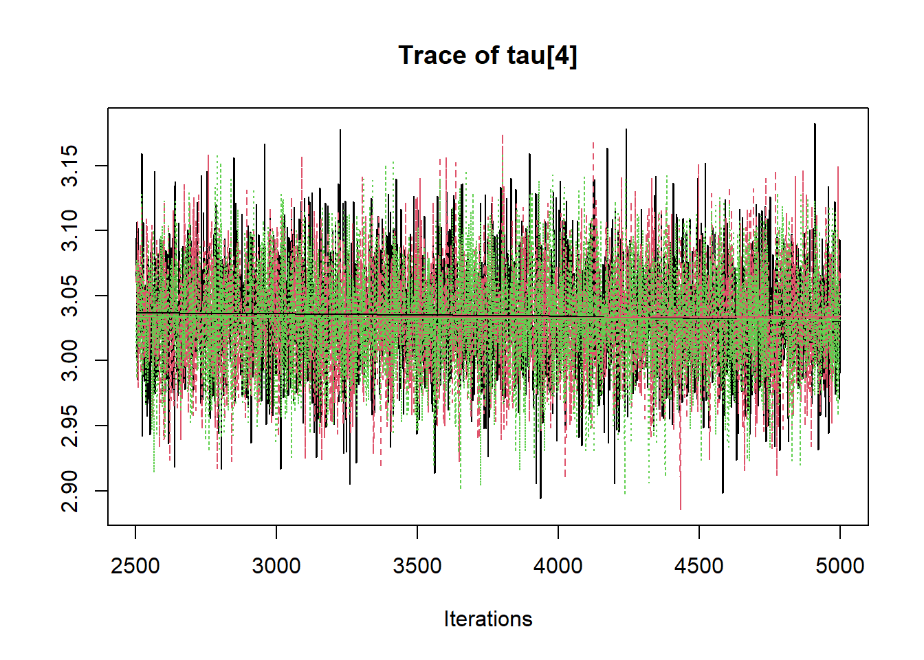
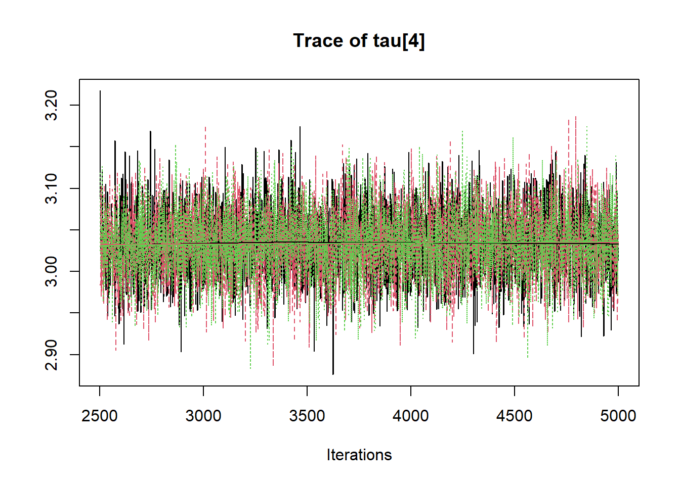
## tau[4] 3.033 0.042 2.953 3.005 3.033 3.062 3.116 1.001 4400
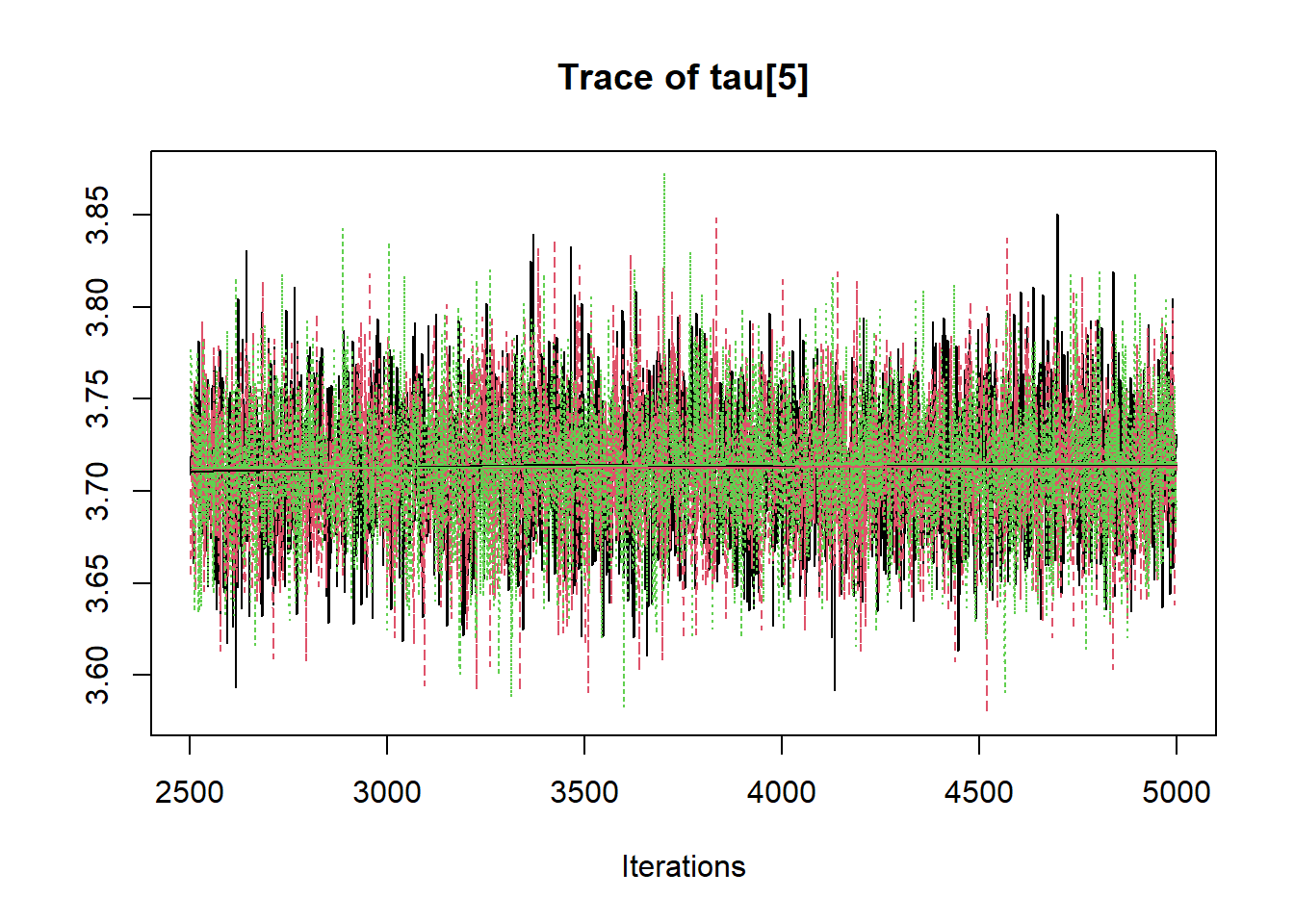
## tau[5] 3.712 0.037 3.639 3.688 3.712 3.737 3.784 1.001 7500
## deviance 3379.989 42.451 3297.778 3351.818 3379.183 3408.556 3465.562 1.001 7500
##
## For each parameter, n.eff is a crude measure of effective sample size,
## and Rhat is the potential scale reduction factor (at convergence, Rhat=1).
##
## DIC info (using the rule, pD = var(deviance)/2)
## pD = 901.2 and DIC = 4281.2
## DIC is an estimate of expected predictive error (lower deviance is better).
# extract posteriors for all chains
jags.mcmc <- as.mcmc(fit)
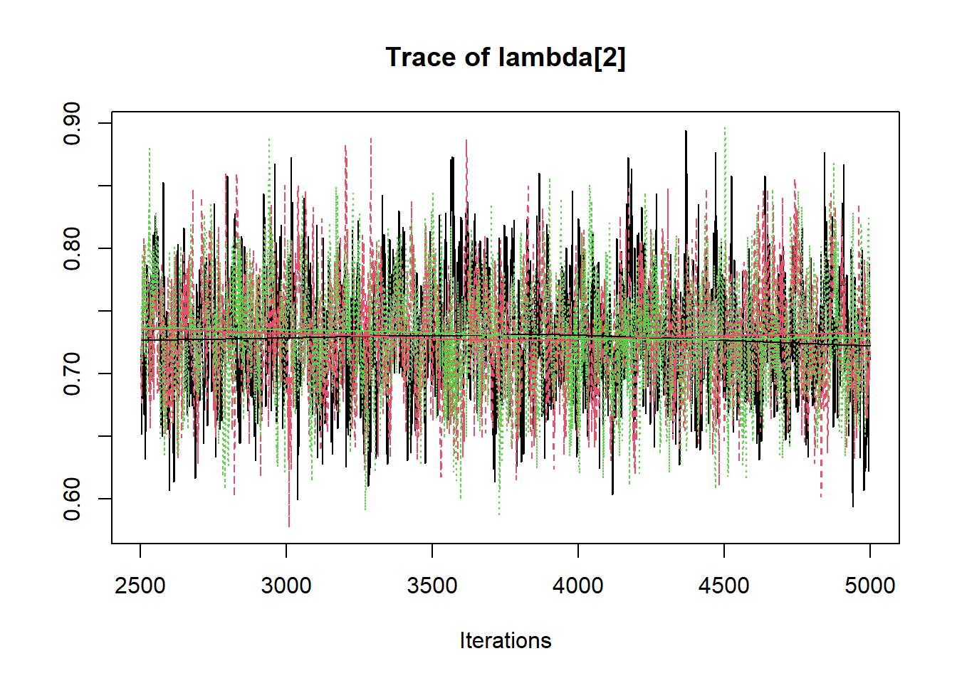
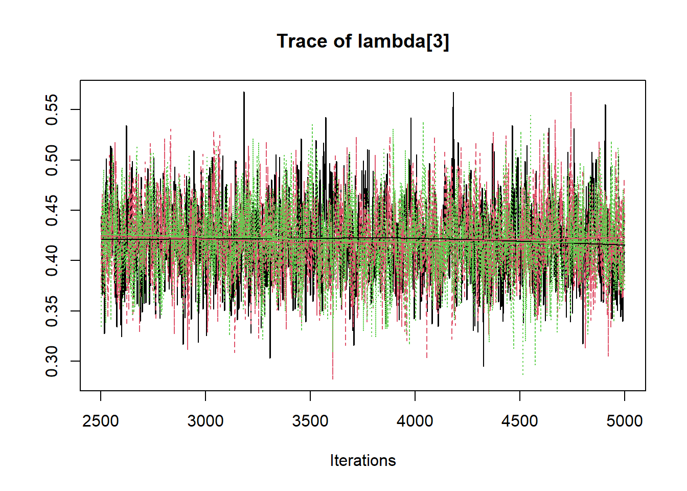
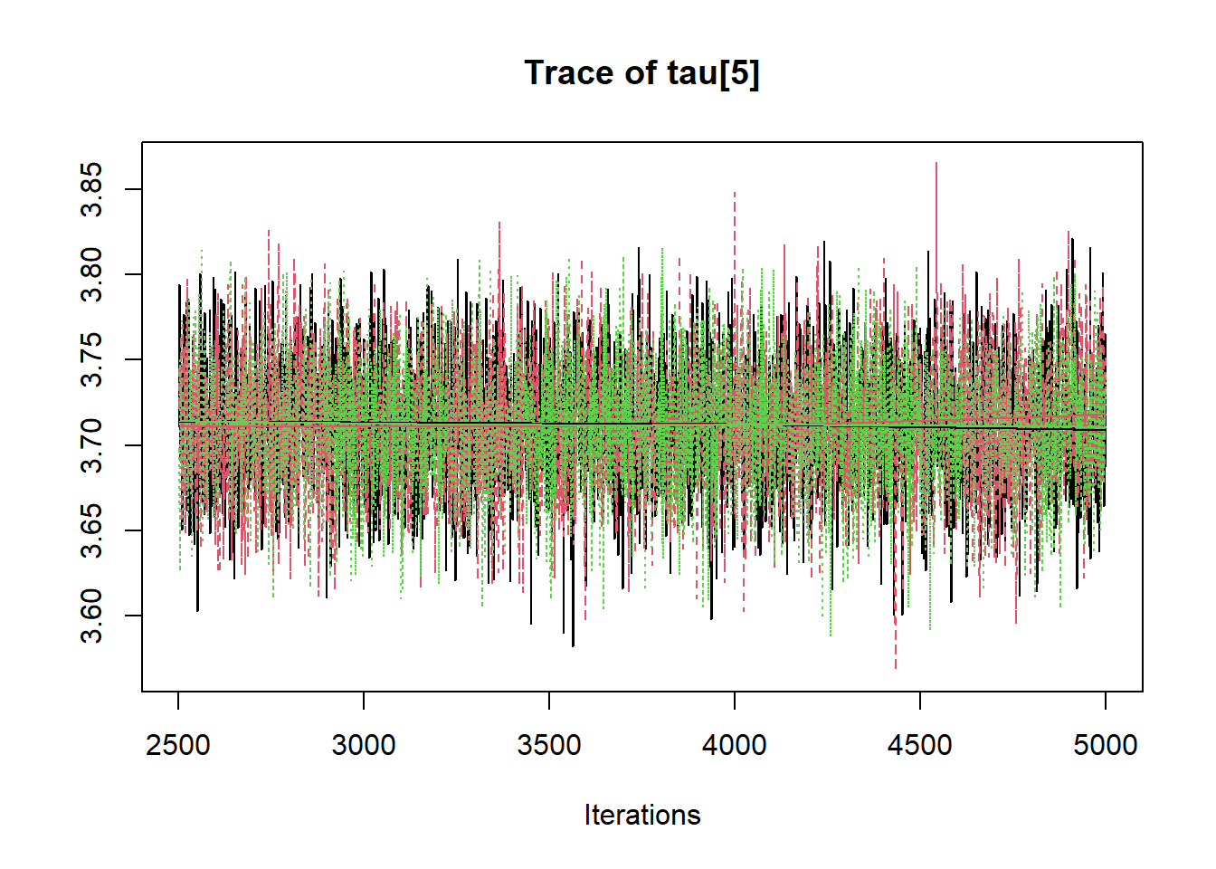
R2jags::traceplot(jags.mcmc)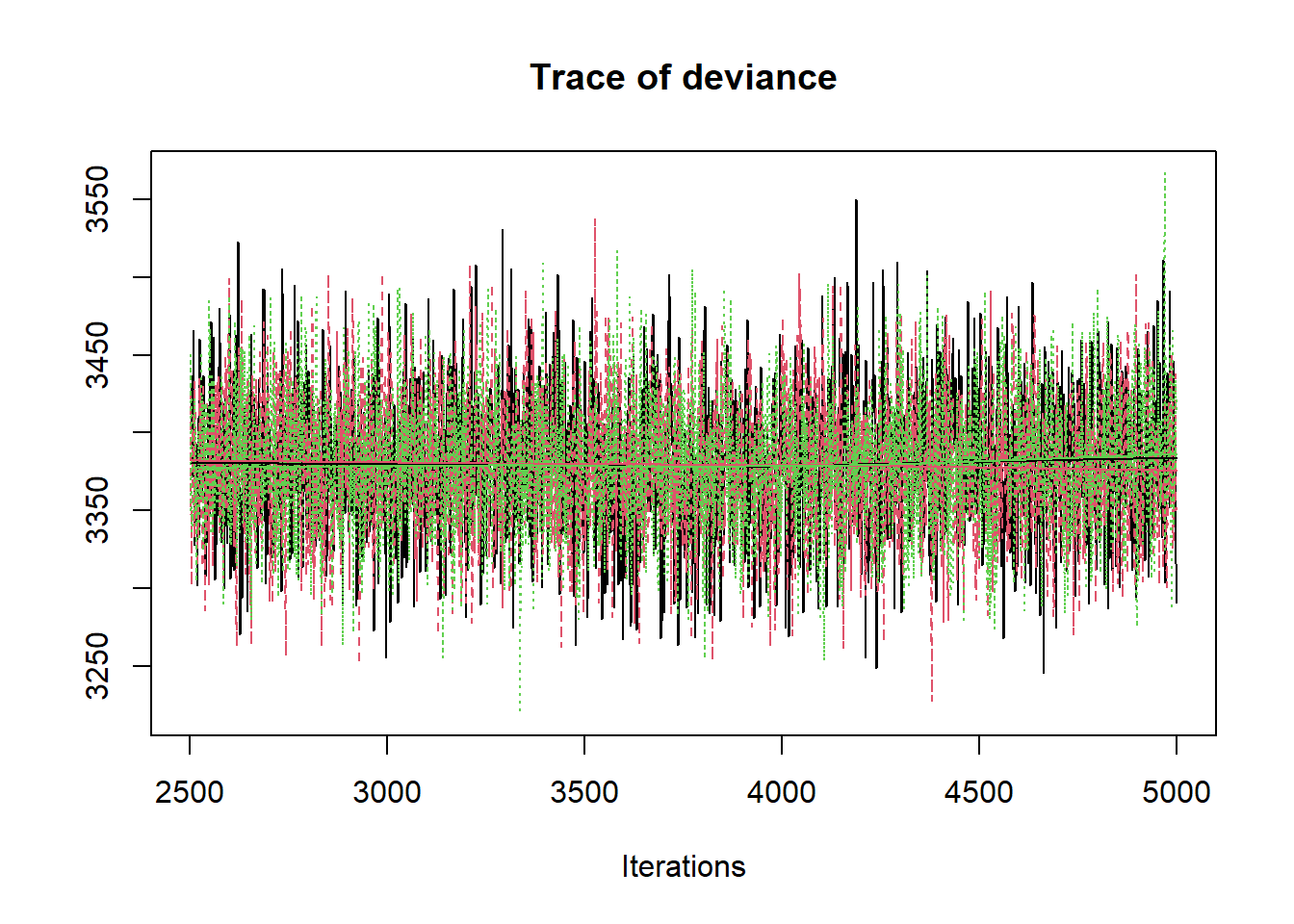
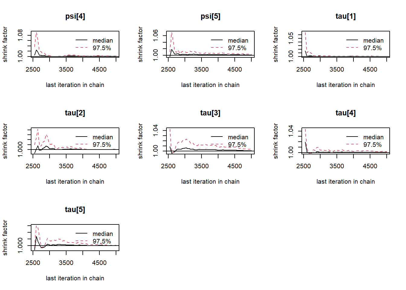
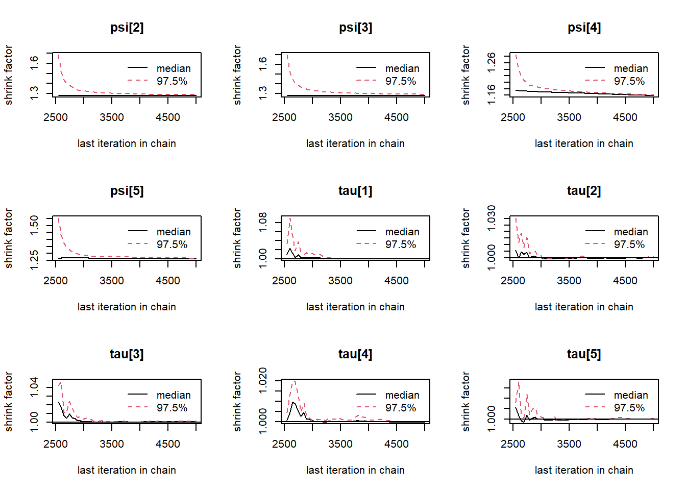
# gelman-rubin-brook
gelman.plot(jags.mcmc)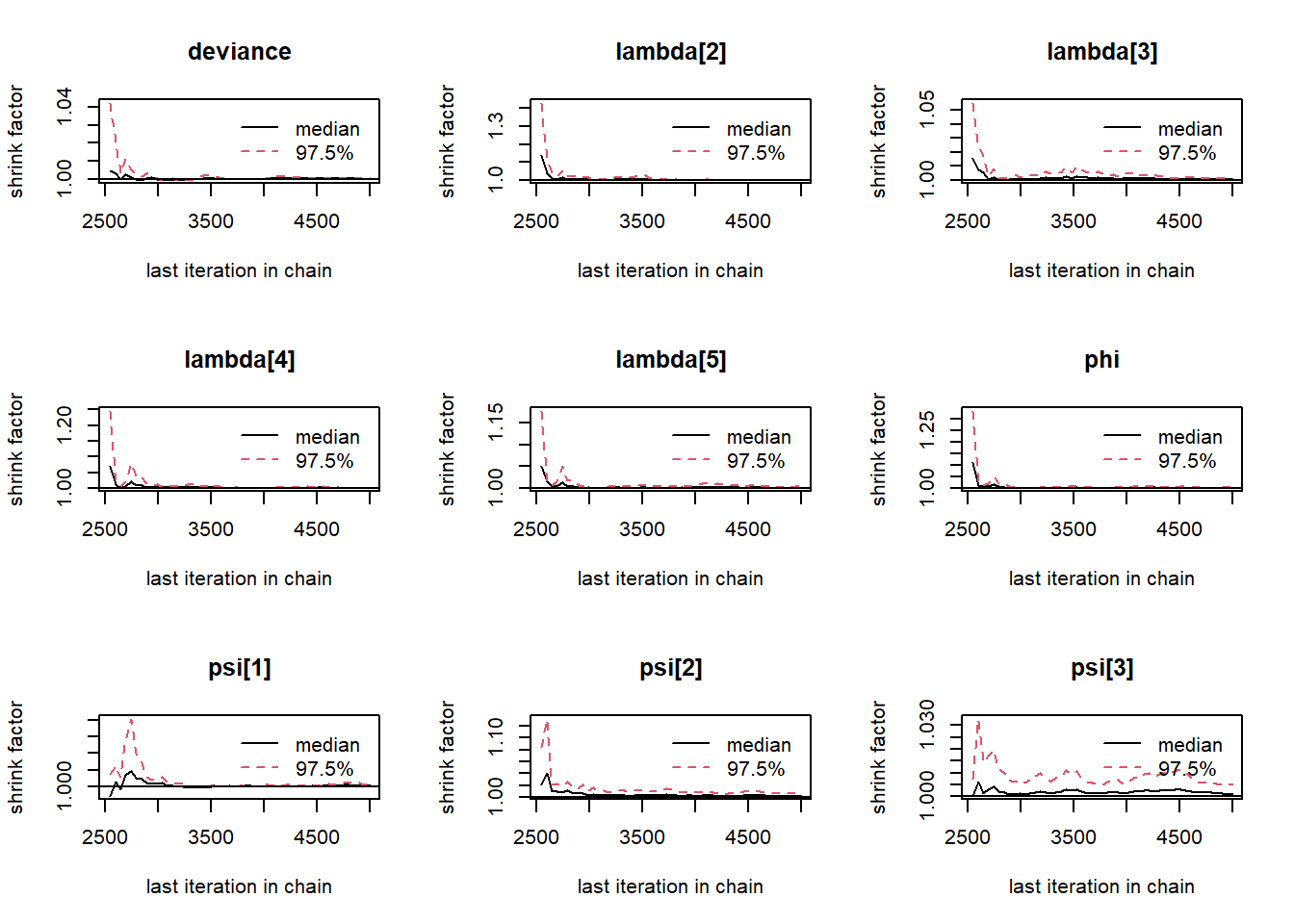
# convert to single data.frame for density plot
a <- colnames(as.data.frame(jags.mcmc[[1]]))
plot.data <- data.frame(as.matrix(jags.mcmc, chains=T, iters = T))
colnames(plot.data) <- c("chain", "iter", a)


plot_title <- ggtitle("Posterior distributions",
                      "with medians and 80% intervals")
mcmc_areas(
  plot.data,
  pars = c(paste0("tau[",1:5,"]")),
  prob = 0.8) +
  plot_title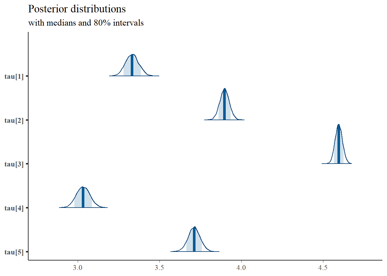
9.3 Stan - Single Latent Variable
model_cfa1 <- '
data {
  int  N;
  int  J;
  matrix[N, J] X;
}

parameters {
  real ksi[N]; //latent variable values
  real tau[J]; //intercepts
  real load[J-1]; //factor loadings
  real<lower=0> psi[J]; //residual variance
  //real kappa; // factor means
  real<lower=0> phi; // factor variances
}

transformed parameters {
  real lambda[J];
  lambda[1] = 1;
  lambda[2:J] = load;
}

model {
  real kappa;
  kappa = 0;
  // likelihood for data
  for(i in 1:N){
    for(j in 1:J){
      X[i, j] ~ normal(tau[j] + ksi[i]*lambda[j], psi[j]);
    }
  }
  // prior for latent variable parameters
  ksi ~ normal(kappa, phi);

  phi ~ inv_gamma(5, 10);
  // prior for measurement model parameters
  tau ~ normal(3, 10);
  psi ~ inv_gamma(5, 10);

  for(j in 1:(J-1)){
    load[j] ~ normal(1, 10);
  }

}

'
# data must be in a list
dat <- read.table("code/CFA-One-Latent-Variable/Data/IIS.dat", header=T)

mydata <- list(
  N = 500, J = 5,
  X = as.matrix(dat)
)

# initial values
start_values <- list(
  list(tau = c(.1,.1,.1,.1,.1), lambda=c(0, 0, 0, 0, 0), phi = 1, psi=c(1, 1, 1, 1, 1)),
  list(tau = c(3,3,3,3,3), lambda=c(3, 3, 3, 3, 3), phi = 2, psi=c(.5, .5, .5, .5, .5)),
  list(tau = c(5, 5, 5, 5, 5), lambda=c(6, 6, 6, 6, 6), phi = 2, psi=c(2, 2, 2, 2, 2))
)

# Next, need to fit the model
#   I have explicitly outlined some common parameters
fit <- stan(
  model_code = model_cfa1, # model code to be compiled
  data = mydata,          # my data
  init = start_values,    # starting values
  chains = 3,             # number of Markov chains
  warmup = 1000,          # number of warm up iterations per chain
  iter = 5000,            # total number of iterations per chain
  cores = 1,              # number of cores (could use one per chain)
  refresh = 0             # no progress shown
)

# first get a basic breakdown of the posteriors
print(fit,pars =c("lambda", "tau", "psi", "phi", "ksi[1]", "ksi[8]"))
## Inference for Stan model: anon_model.
## 3 chains, each with iter=5000; warmup=1000; thin=1;
## post-warmup draws per chain=4000, total post-warmup draws=12000.
##
## mean se_mean sd 2.5% 25% 50% 75% 97.5% n_eff Rhat
## lambda[1] 1.00 NaN 0.00 1.00 1.00 1.00 1.00 1.00 NaN NaN
## lambda[2] 0.81 0 0.05 0.72 0.78 0.81 0.85 0.92 1491 1
## lambda[3] 0.47 0 0.04 0.40 0.45 0.47 0.50 0.55 2377 1
## lambda[4] 1.10 0 0.07 0.97 1.05 1.10 1.15 1.26 1682 1
## lambda[5] 1.06 0 0.07 0.93 1.01 1.06 1.10 1.20 1491 1
## tau[1] 3.33 0 0.04 3.26 3.31 3.33 3.36 3.41 2409 1
## tau[2] 3.90 0 0.03 3.84 3.88 3.90 3.92 3.95 2080 1
## tau[3] 4.60 0 0.02 4.55 4.58 4.60 4.61 4.64 3140 1
## tau[4] 3.03 0 0.04 2.96 3.01 3.03 3.06 3.11 2329 1
## tau[5] 3.71 0 0.04 3.64 3.69 3.71 3.74 3.78 2098 1
## psi[1] 0.60 0 0.02 0.55 0.58 0.60 0.61 0.64 8087 1
## psi[2] 0.36 0 0.02 0.33 0.35 0.36 0.37 0.40 4521 1
## psi[3] 0.37 0 0.01 0.35 0.37 0.37 0.38 0.40 9691 1
## psi[4] 0.60 0 0.02 0.56 0.59 0.60 0.62 0.65 7454 1
## psi[5] 0.48 0 0.02 0.44 0.47 0.48 0.50 0.52 5708 1
## phi 0.60 0 0.03 0.54 0.58 0.60 0.62 0.67 1459 1
## ksi[1] -0.23 0 0.22 -0.67 -0.38 -0.23 -0.08 0.21 18018 1
## ksi[8] 0.85 0 0.23 0.41 0.69 0.84 0.99 1.30 11586 1
##
## Samples were drawn using NUTS(diag_e) at Mon Jun 20 03:38:56 2022.
## For each parameter, n_eff is a crude measure of effective sample size,
## and Rhat is the potential scale reduction factor on split chains (at
## convergence, Rhat=1).
# plot the posterior in a
#  95% probability interval
#  and 80% to contrast the dispersion
plot(fit,pars =c("lambda", "tau", "psi", "phi", "ksi[1]", "ksi[8]"))
## ci_level: 0.8 (80% intervals)## outer_level: 0.95 (95% intervals)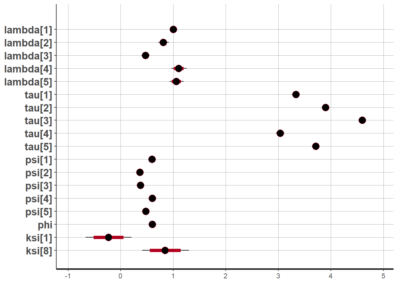
# traceplots
rstan::traceplot(fit,pars =c("lambda", "tau", "psi", "phi", "ksi[1]", "ksi[8]"), inc_warmup = TRUE)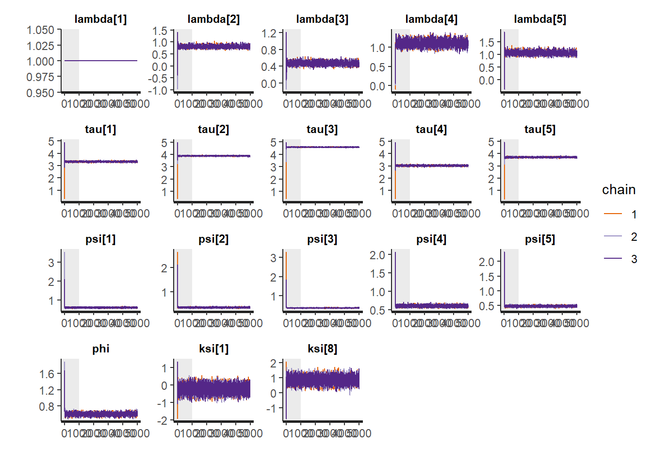
# Gelman-Rubin-Brooks Convergence Criterion
ggs_grb(ggs(fit, family = c("lambda"))) +
   theme_bw() + theme(panel.grid = element_blank())
## Warning: Removed 50 row(s) containing missing values (geom_path).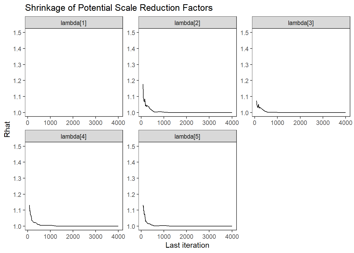
ggs_grb(ggs(fit, family = "tau")) +
   theme_bw() + theme(panel.grid = element_blank())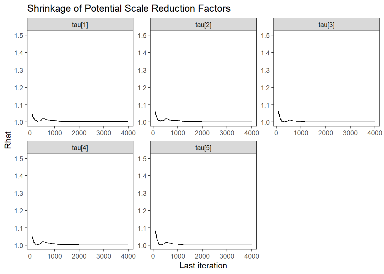
ggs_grb(ggs(fit, family = "psi")) +
   theme_bw() + theme(panel.grid = element_blank())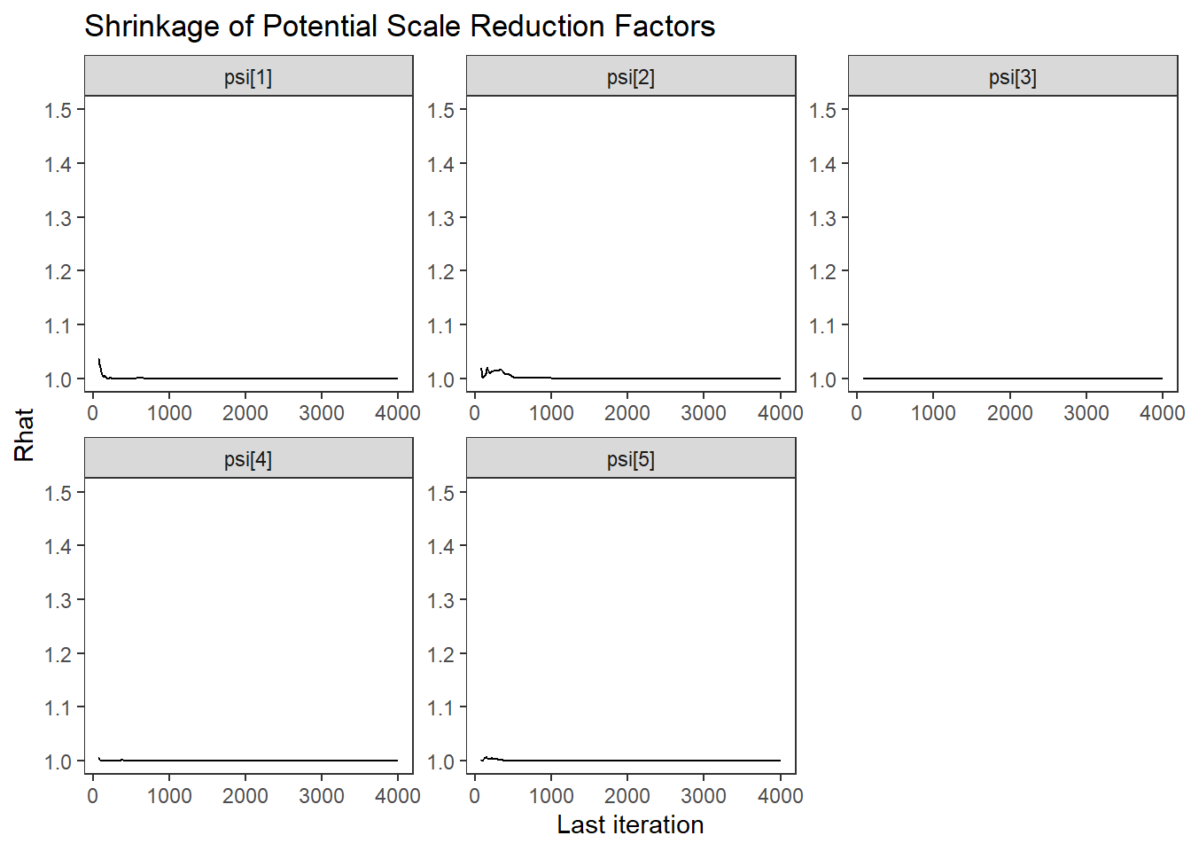
ggs_grb(ggs(fit, family = "phi")) +
   theme_bw() + theme(panel.grid = element_blank())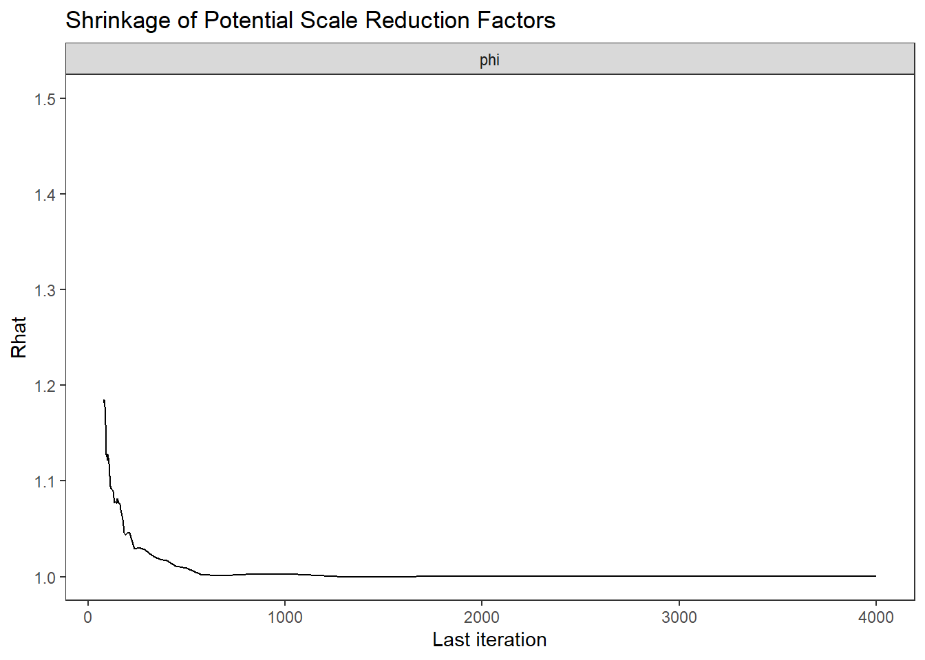
# autocorrelation
ggs_autocorrelation(ggs(fit, family="lambda")) +
   theme_bw() + theme(panel.grid = element_blank())
## Warning in cor(X, use = "pairwise.complete.obs"): the standard deviation is zero## Warning in cor(X, use = "pairwise.complete.obs"): the standard deviation is zero
## Warning in cor(X, use = "pairwise.complete.obs"): the standard deviation is zero## Warning: Removed 150 rows containing missing values (geom_bar).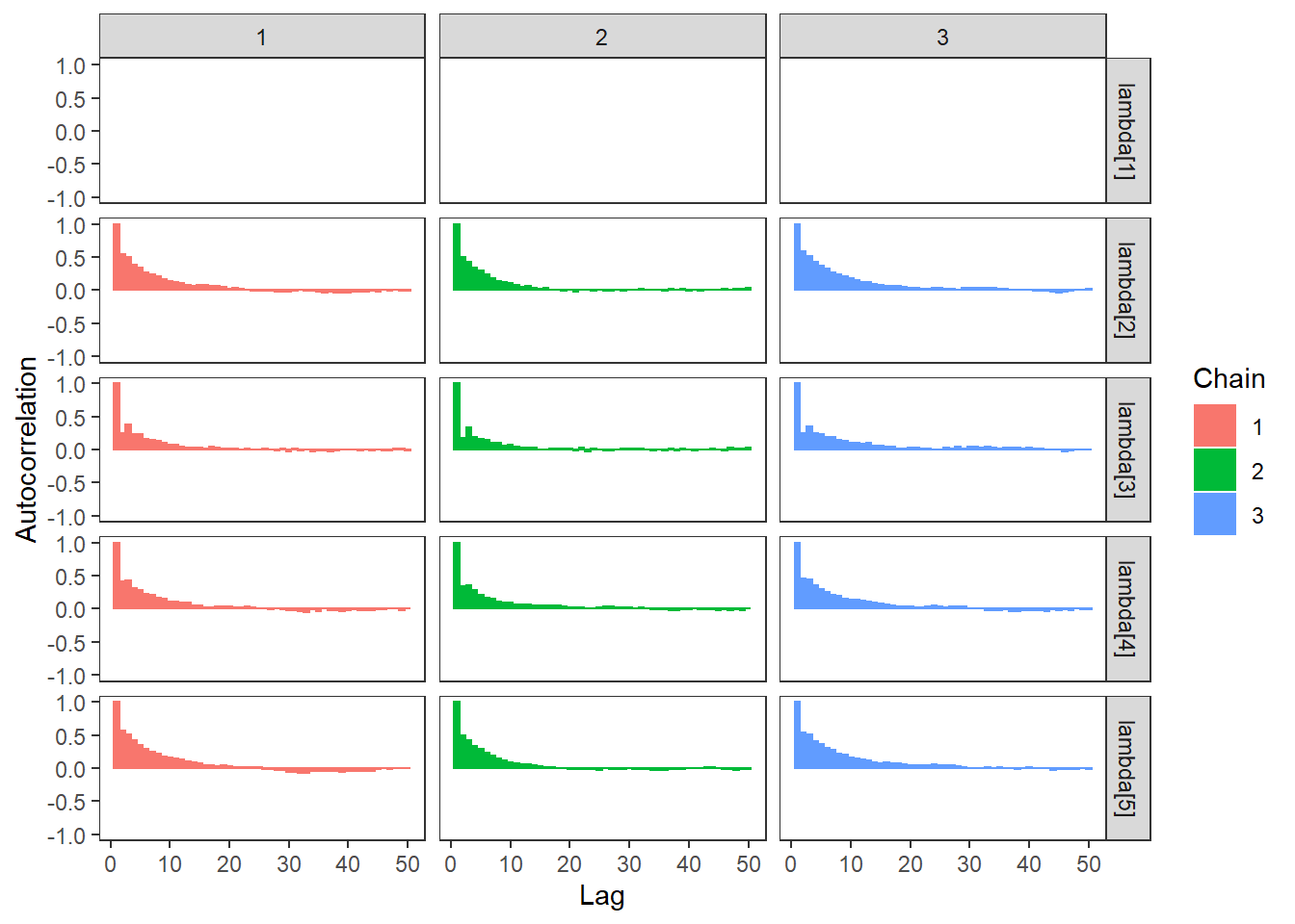
ggs_autocorrelation(ggs(fit, family="tau")) +
   theme_bw() + theme(panel.grid = element_blank())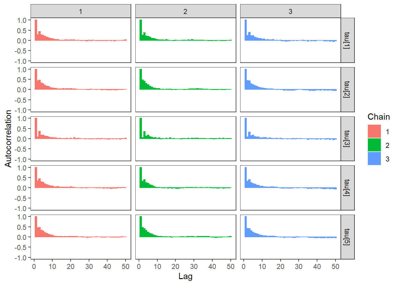
ggs_autocorrelation(ggs(fit, family="psi")) +
   theme_bw() + theme(panel.grid = element_blank())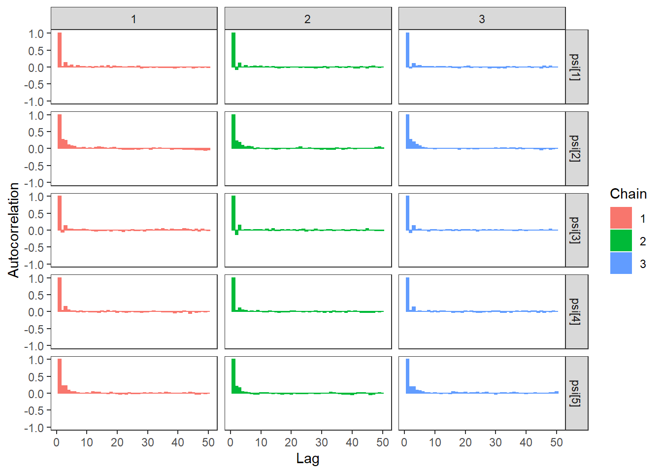
ggs_autocorrelation(ggs(fit, family="phi")) +
   theme_bw() + theme(panel.grid = element_blank())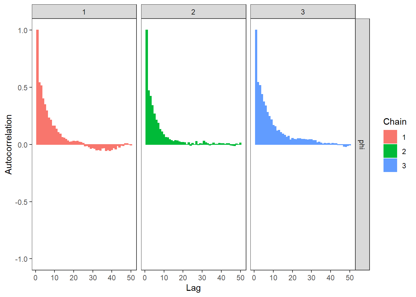
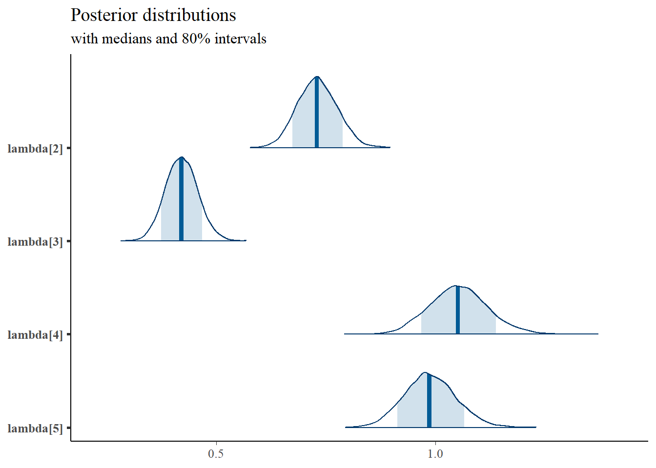
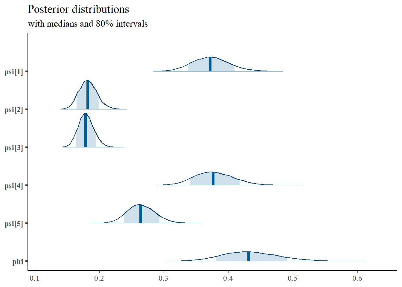
# plot the posterior density
plot.data <- as.matrix(fit)

plot_title <- ggtitle("Posterior distributions",
                      "with medians and 80% intervals")
mcmc_areas(
  plot.data,
  pars = paste0("lambda[",1:5,"]"),
  prob = 0.8) +
  plot_title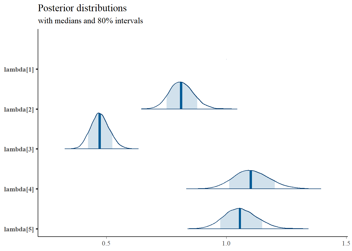
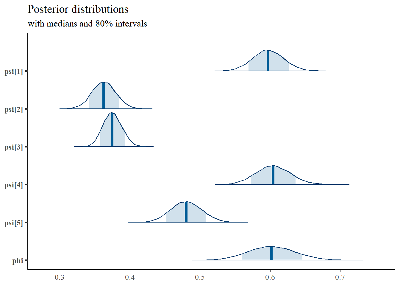
mcmc_areas(
  plot.data,
  pars = paste0("tau[",1:5,"]"),
  prob = 0.8) +
  plot_title
# I prefer a posterior plot that includes prior and MLE
# Expanded Posterior Plot
colnames(dat) <- paste0("x",1:5)
lav.mod <- '
  xi =~ 1*x1 + x2 + x3 + x4 + x5
  xi ~~ xi
  x1 ~ 1
  x2 ~ 1
  x3 ~ 1
  x4 ~ 1
  x5 ~ 1
'
lav.fit <- lavaan::cfa(lav.mod, data=dat)

MLE <- lavaan::parameterEstimates(lav.fit)

prior_tau <- function(x){dnorm(x, 3, 10)}
x.tau<- seq(1, 5, 0.01)
prior.tau <- data.frame(tau=x.tau, dens.mtau = prior_tau(x.tau))

prior_lambda <- function(x){dnorm(x, 1, 10)}
x.lambda<- seq(0, 2, 0.01)
prior.lambda <- data.frame(lambda=x.lambda, dens.lambda = prior_lambda(x.lambda))

prior_sig <- function(x){dinvgamma(x, 5, 10)}
x.sig<- seq(.01, 1, 0.01)
prior.sig <- data.frame(sig=x.sig, dens.sig = prior_sig(x.sig))

prior_sige <- function(x){dinvgamma(x, 1, 4)}
x.sige<- seq(.1, 10, 0.1)
prior.sige <- data.frame(sige=x.sige, dens.sige = prior_sige(x.sige))

prior_ksi <- function(x){
  mu <- 0
  sig <- rinvgamma(1, 5, 10)
  rnorm(x, mu, sig)
}
x.ksi<- seq(-5, 5, 0.01)
prior.ksi <- data.frame(ksi=prior_ksi(10000))

cols <- c("Posterior"="#0072B2", "Prior"="#E69F00", "MLE"= "black")#"#56B4E9", "#E69F00" "#CC79A7"

# get stan samples
plot.data <- as.data.frame(plot.data)

# make plotting pieces
p1 <- ggplot()+
  geom_density(data=plot.data,
               aes(x=`lambda[1]`, color="Posterior"))+
  geom_line(data=prior.lambda,
            aes(x=lambda, y=dens.lambda, color="Prior"))+
  geom_vline(aes(xintercept=MLE[1, 4], color="MLE"))+
  scale_color_manual(values=cols, name=NULL)+
  lims(x=c(0.25, 1.5))+
  theme_bw()+
  theme(panel.grid = element_blank())
p2 <- ggplot()+
  geom_density(data=plot.data,
               aes(x=`lambda[2]`, color="Posterior"))+
  geom_line(data=prior.lambda,
            aes(x=lambda, y=dens.lambda, color="Prior"))+
  geom_vline(aes(xintercept=MLE[2, 4], color="MLE"))+
  scale_color_manual(values=cols, name=NULL)+
  lims(x=c(0.25, 1.5))+
  theme_bw()+
  theme(panel.grid = element_blank())
p3 <- ggplot()+
  geom_density(data=plot.data,
               aes(x=`lambda[3]`, color="Posterior"))+
  geom_line(data=prior.lambda,
            aes(x=lambda, y=dens.lambda, color="Prior"))+
  geom_vline(aes(xintercept=MLE[3, 4], color="MLE"))+
  scale_color_manual(values=cols, name=NULL)+
  lims(x=c(0.25, 1.5))+
  theme_bw()+
  theme(panel.grid = element_blank())
p4 <- ggplot()+
  geom_density(data=plot.data,
               aes(x=`lambda[4]`, color="Posterior"))+
  geom_line(data=prior.lambda,
            aes(x=lambda, y=dens.lambda, color="Prior"))+
  geom_vline(aes(xintercept=MLE[4, 4], color="MLE"))+
  scale_color_manual(values=cols, name=NULL)+
  lims(x=c(0.25, 1.5))+
  theme_bw()+
  theme(panel.grid = element_blank())
p5 <- ggplot()+
  geom_density(data=plot.data,
               aes(x=`lambda[5]`, color="Posterior"))+
  geom_line(data=prior.lambda,
            aes(x=lambda, y=dens.lambda, color="Prior"))+
  geom_vline(aes(xintercept=MLE[5, 4], color="MLE"))+
  scale_color_manual(values=cols, name=NULL)+
  lims(x=c(0.25, 1.5))+theme_bw()+
  theme(panel.grid = element_blank())
p1 + p2 + p3 + p4 + p5 + plot_layout(guides="collect")
## Warning: Removed 75 row(s) containing missing values (geom_path).## Warning: Removed 75 row(s) containing missing values (geom_path).
## Removed 75 row(s) containing missing values (geom_path).
## Removed 75 row(s) containing missing values (geom_path).
## Removed 75 row(s) containing missing values (geom_path).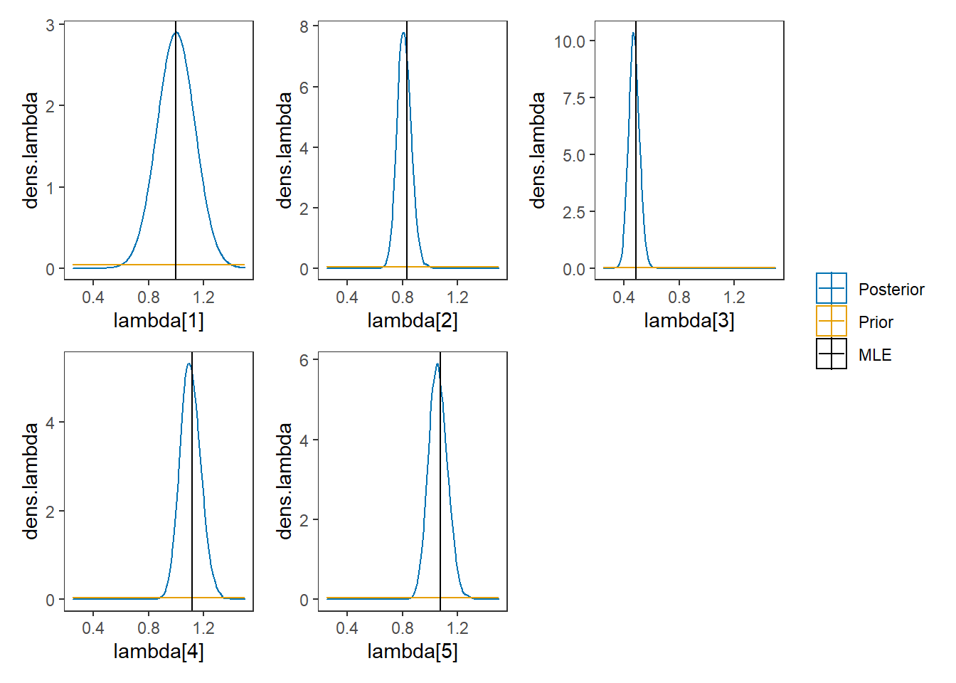
# phi
p1 <- ggplot()+
  geom_density(data=plot.data,
               aes(x=`phi`, color="Posterior"))+
  geom_line(data=prior.sig,
            aes(x=sig, y=dens.sig, color="Prior"))+
  geom_vline(aes(xintercept=sqrt(MLE[6,4]), color="MLE"))+
  scale_color_manual(values=cols, name=NULL)+
  theme_bw()+
  theme(panel.grid = element_blank())

# psi
p2 <- ggplot()+
  geom_density(data=plot.data,
               aes(x=`psi[1]`, color="Posterior"))+
  geom_line(data=prior.sig,
            aes(x=sig, y=dens.sig, color="Prior"))+
  geom_vline(aes(xintercept=sqrt(MLE[12,4]), color="MLE"))+
  scale_color_manual(values=cols, name=NULL)+
  theme_bw()+
  theme(panel.grid = element_blank())
p3 <- ggplot()+
  geom_density(data=plot.data,
               aes(x=`psi[2]`, color="Posterior"))+
  geom_line(data=prior.sig,
            aes(x=sig, y=dens.sig, color="Prior"))+
  geom_vline(aes(xintercept=sqrt(MLE[13,4]), color="MLE"))+
  scale_color_manual(values=cols, name=NULL)+
  theme_bw()+
  theme(panel.grid = element_blank())
p4 <- ggplot()+
  geom_density(data=plot.data,
               aes(x=`psi[3]`, color="Posterior"))+
  geom_line(data=prior.sig,
            aes(x=sig, y=dens.sig, color="Prior"))+
  geom_vline(aes(xintercept=sqrt(MLE[14,4]), color="MLE"))+
  scale_color_manual(values=cols, name=NULL)+
  theme_bw()+
  theme(panel.grid = element_blank())
p5 <- ggplot()+
  geom_density(data=plot.data,
               aes(x=`psi[4]`, color="Posterior"))+
  geom_line(data=prior.sig,
            aes(x=sig, y=dens.sig, color="Prior"))+
  geom_vline(aes(xintercept=sqrt(MLE[15,4]), color="MLE"))+
  scale_color_manual(values=cols, name=NULL)+
  theme_bw()+
  theme(panel.grid = element_blank())
p6 <- ggplot()+
  geom_density(data=plot.data,
               aes(x=`psi[5]`, color="Posterior"))+
  geom_line(data=prior.sig,
            aes(x=sig, y=dens.sig, color="Prior"))+
  geom_vline(aes(xintercept=sqrt(MLE[16,4]), color="MLE"))+
  scale_color_manual(values=cols, name=NULL)+
  theme_bw()+
  theme(panel.grid = element_blank())

p1 + p2 + p3 + p4 + p5 + p6 + plot_layout(guides = "collect")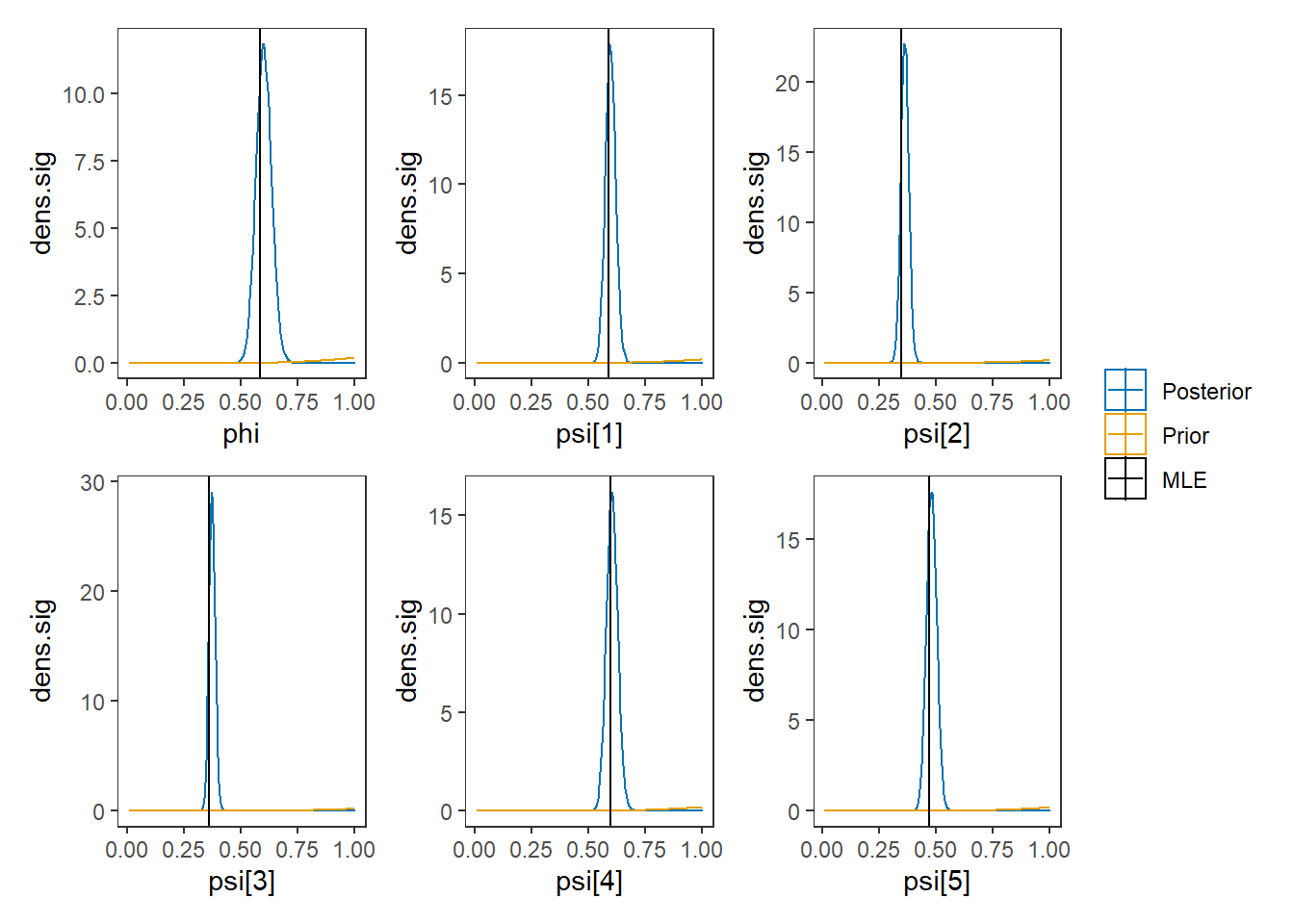
9.4 Blavaan - Single Latent Variable
# model
model_cfa_blavaan <- "
  f1 =~ 1*PI + AD + IGC + FI + FC
"

dat <- as.matrix(read.table("code/CFA-Two-Latent-Variables/Data/IIS.dat", header=T))

fit <- blavaan::bcfa(model_cfa_blavaan, data=dat)
##
## SAMPLING FOR MODEL 'stanmarg' NOW (CHAIN 1).
## Chain 1:
## Chain 1: Gradient evaluation took 0.001 seconds
## Chain 1: 1000 transitions using 10 leapfrog steps per transition would take 10 seconds.
## Chain 1: Adjust your expectations accordingly!
## Chain 1:
## Chain 1:
## Chain 1: Iteration: 1 / 1500 [ 0%] (Warmup)
## Chain 1: Iteration: 150 / 1500 [ 10%] (Warmup)
## Chain 1: Iteration: 300 / 1500 [ 20%] (Warmup)
## Chain 1: Iteration: 450 / 1500 [ 30%] (Warmup)
## Chain 1: Iteration: 501 / 1500 [ 33%] (Sampling)
## Chain 1: Iteration: 650 / 1500 [ 43%] (Sampling)
## Chain 1: Iteration: 800 / 1500 [ 53%] (Sampling)
## Chain 1: Iteration: 950 / 1500 [ 63%] (Sampling)
## Chain 1: Iteration: 1100 / 1500 [ 73%] (Sampling)
## Chain 1: Iteration: 1250 / 1500 [ 83%] (Sampling)
## Chain 1: Iteration: 1400 / 1500 [ 93%] (Sampling)
## Chain 1: Iteration: 1500 / 1500 [100%] (Sampling)
## Chain 1:
## Chain 1: Elapsed Time: 2.778 seconds (Warm-up)
## Chain 1: 5.302 seconds (Sampling)
## Chain 1: 8.08 seconds (Total)
## Chain 1:
##
## SAMPLING FOR MODEL 'stanmarg' NOW (CHAIN 2).
## Chain 2:
## Chain 2: Gradient evaluation took 0 seconds
## Chain 2: 1000 transitions using 10 leapfrog steps per transition would take 0 seconds.
## Chain 2: Adjust your expectations accordingly!
## Chain 2:
## Chain 2:
## Chain 2: Iteration: 1 / 1500 [ 0%] (Warmup)
## Chain 2: Iteration: 150 / 1500 [ 10%] (Warmup)
## Chain 2: Iteration: 300 / 1500 [ 20%] (Warmup)
## Chain 2: Iteration: 450 / 1500 [ 30%] (Warmup)
## Chain 2: Iteration: 501 / 1500 [ 33%] (Sampling)
## Chain 2: Iteration: 650 / 1500 [ 43%] (Sampling)
## Chain 2: Iteration: 800 / 1500 [ 53%] (Sampling)
## Chain 2: Iteration: 950 / 1500 [ 63%] (Sampling)
## Chain 2: Iteration: 1100 / 1500 [ 73%] (Sampling)
## Chain 2: Iteration: 1250 / 1500 [ 83%] (Sampling)
## Chain 2: Iteration: 1400 / 1500 [ 93%] (Sampling)
## Chain 2: Iteration: 1500 / 1500 [100%] (Sampling)
## Chain 2:
## Chain 2: Elapsed Time: 2.809 seconds (Warm-up)
## Chain 2: 5.188 seconds (Sampling)
## Chain 2: 7.997 seconds (Total)
## Chain 2:
##
## SAMPLING FOR MODEL 'stanmarg' NOW (CHAIN 3).
## Chain 3:
## Chain 3: Gradient evaluation took 0 seconds
## Chain 3: 1000 transitions using 10 leapfrog steps per transition would take 0 seconds.
## Chain 3: Adjust your expectations accordingly!
## Chain 3:
## Chain 3:
## Chain 3: Iteration: 1 / 1500 [ 0%] (Warmup)
## Chain 3: Iteration: 150 / 1500 [ 10%] (Warmup)
## Chain 3: Iteration: 300 / 1500 [ 20%] (Warmup)
## Chain 3: Iteration: 450 / 1500 [ 30%] (Warmup)
## Chain 3: Iteration: 501 / 1500 [ 33%] (Sampling)
## Chain 3: Iteration: 650 / 1500 [ 43%] (Sampling)
## Chain 3: Iteration: 800 / 1500 [ 53%] (Sampling)
## Chain 3: Iteration: 950 / 1500 [ 63%] (Sampling)
## Chain 3: Iteration: 1100 / 1500 [ 73%] (Sampling)
## Chain 3: Iteration: 1250 / 1500 [ 83%] (Sampling)
## Chain 3: Iteration: 1400 / 1500 [ 93%] (Sampling)
## Chain 3: Iteration: 1500 / 1500 [100%] (Sampling)
## Chain 3:
## Chain 3: Elapsed Time: 2.751 seconds (Warm-up)
## Chain 3: 5.192 seconds (Sampling)
## Chain 3: 7.943 seconds (Total)
## Chain 3:
## Computing posterior predictives...
summary(fit)## blavaan (0.4-3) results of 1000 samples after 500 adapt/burnin iterations
##
## Number of observations 500
##
## Number of missing patterns 1
##
## Statistic MargLogLik PPP
## Value -2196.532 0.000
##
## Latent Variables:
## Estimate Post.SD pi.lower pi.upper Rhat Prior
## f1 =~
## PI 1.000
## AD 0.847 0.056 0.743 0.964 1.002 normal(0,10)
## IGC 0.494 0.043 0.414 0.579 1.003 normal(0,10)
## FI 1.131 0.079 0.984 1.298 1.003 normal(0,10)
## FC 1.090 0.074 0.955 1.252 1.003 normal(0,10)
##
## Intercepts:
## Estimate Post.SD pi.lower pi.upper Rhat Prior
## .PI 3.332 0.038 3.253 3.407 1.000 normal(0,32)
## .AD 3.896 0.028 3.840 3.950 1.000 normal(0,32)
## .IGC 4.595 0.022 4.554 4.638 1.000 normal(0,32)
## .FI 3.032 0.042 2.952 3.112 1.000 normal(0,32)
## .FC 3.711 0.037 3.637 3.783 1.000 normal(0,32)
## f1 0.000
##
## Variances:
## Estimate Post.SD pi.lower pi.upper Rhat Prior
## .PI 0.353 0.026 0.305 0.407 1.001 gamma(1,.5)[sd]
## .AD 0.120 0.012 0.097 0.145 1.000 gamma(1,.5)[sd]
## .IGC 0.133 0.009 0.115 0.152 1.002 gamma(1,.5)[sd]
## .FI 0.363 0.030 0.307 0.422 1.001 gamma(1,.5)[sd]
## .FC 0.224 0.021 0.185 0.269 1.000 gamma(1,.5)[sd]
## f1 0.337 0.041 0.259 0.423 1.002 gamma(1,.5)[sd]
plot(fit)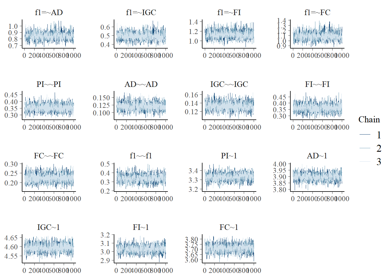
9.5 Two Latent Variable Model
Here we consider the model in section 9.4 which is a CFA model with 2 latent variables and 5 observed indicators. The graphical representation of these factor models get pretty complex pretty quickly, but for this example I have reproduced a version of Figure 9.4, shown below.
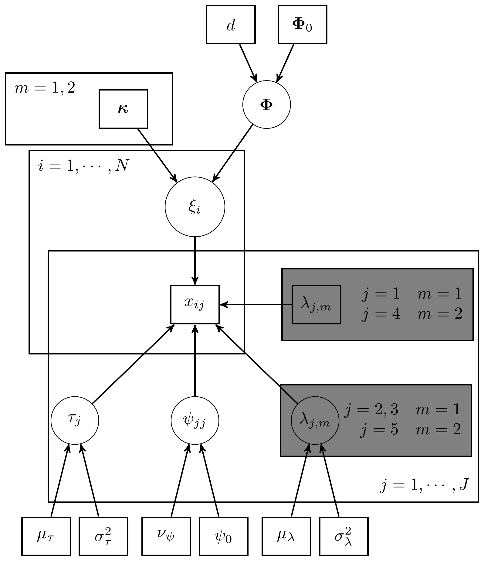
Figure 9.4: DAG for CFA model with 2 latent variables
However, as the authors noted, the path diagram tradition of conveying models is also very useful in discussing and describing the model, which I give next.
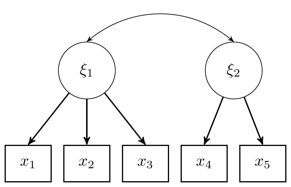
Figure 9.5: Path Diagram for CFA model with 2 latent variables
For completeness, I have included the model specification diagram that more concretely connects the DAG and path diagram to the assumed distributions and priors.
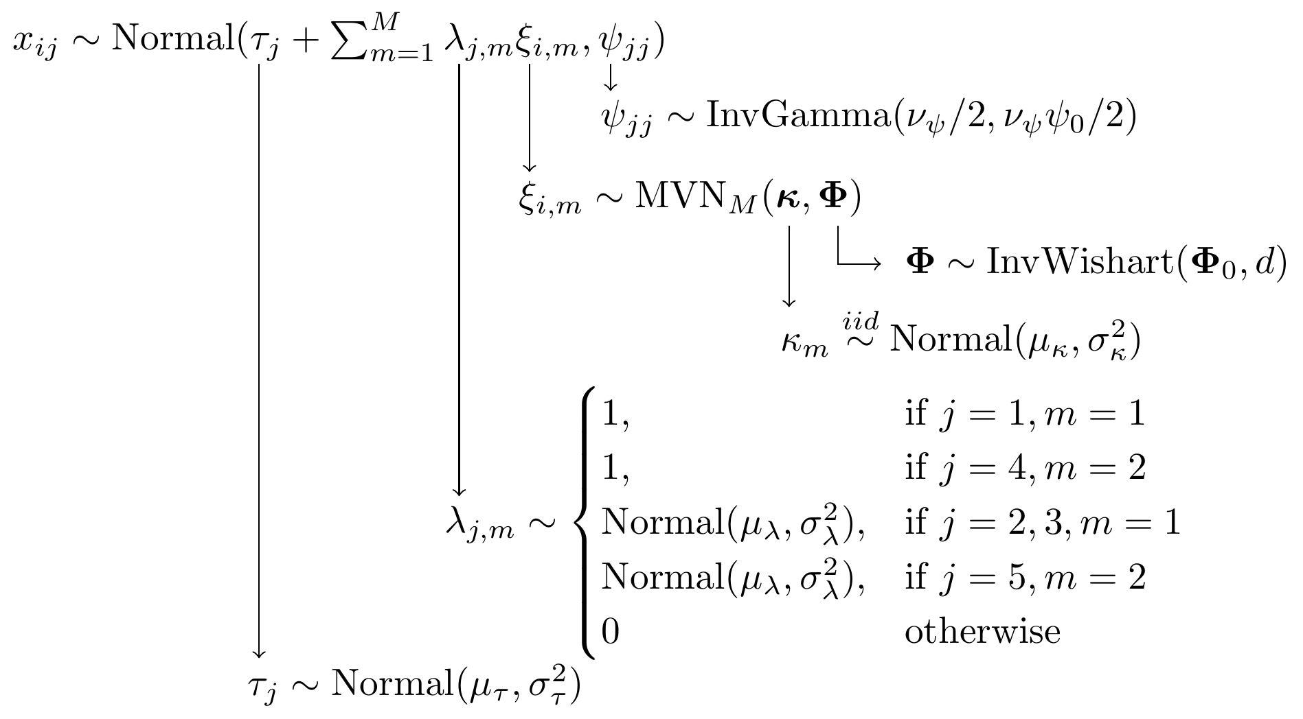
Figure 9.6: Model specification diagram for the CFA model with 2 latent factors
9.6 JAGS - Two Latent Variable
# model code
jags.model.cfa2 <- function(){

  ###################
  # Specify the factor analysis measurement model for the observables
  ####################
  for (i in 1:n){

    # expected value for each examinee for each observable
    mu[i,1] <- tau[1] + lambda[1,1]*ksi[i,1]
    mu[i,2] <- tau[2] + lambda[2,1]*ksi[i,1]
    mu[i,3] <- tau[3] + lambda[3,1]*ksi[i,1]
    mu[i,4] <- tau[4] + lambda[4,2]*ksi[i,2]
    mu[i,5] <- tau[5] + lambda[5,2]*ksi[i,2]

    for(j in 1:J){
      x[i,j] ~ dnorm(mu[i,j], inv.psi[j])    # distribution for each observable
    }
  }


  ######################################################################
  # Specify the (prior) distribution for the latent variables
  ######################################################################
  for (i in 1:n){
    ksi[i, 1:M] ~ dmnorm(kappa[], inv.phi[,])  # distribution for the latent variables
  }


  ######################################################################
  # Specify the prior distribution for the parameters that govern the latent variables
  ######################################################################
  for(m in 1:M){
    kappa[m] <- 0              # Means of latent variables
  }

  inv.phi[1:M,1:M] ~ dwish(dxphi.0[ , ], d);    # prior for precision matrix for the latent variables
  phi[1:M,1:M] <- inverse(inv.phi[ , ]);        # the covariance matrix for the latent vars

  phi.0[1,1] <- 1;
  phi.0[1,2] <- .3;
  phi.0[2,1] <- .3;
  phi.0[2,2] <- 1;
  d <- 2;

  for (m in 1:M){
       for (mm in 1:M){
            dxphi.0[m,mm] <- d*phi.0[m,mm];
       }
  }


  ######################################################################
  # Specify the prior distribution for the measurement model parameters
  ######################################################################
  for(j in 1:J){
    tau[j] ~ dnorm(3, .1)        # Intercepts for observables
    inv.psi[j] ~ dgamma(5, 10) # Precisions for observables
    psi[j] <- 1/inv.psi[j]   # Variances for observables
  }

  lambda[1,1] <- 1.0              # loading fixed to 1.0
  lambda[4,2] <- 1.0              # loading fixed to 1.0

  for (j in 2:3){
    lambda[j,1] ~ dnorm(1, .1)    # prior distribution for the remaining loadings
  }
  lambda[5,2] ~ dnorm(1, .1)      # prior distribution for the remaining loadings
}
# data must be in a list
dat <- read.table("code/CFA-One-Latent-Variable/Data/IIS.dat", header=T)

mydata <- list(
  n = 500, J = 5, M =2,
  x = as.matrix(dat)
)


# initial values
start_values <- list(
  list("tau"=c(1.00E-01, 1.00E-01, 1.00E-01, 1.00E-01, 1.00E-01),
       lambda= structure(
         .Data= c( NA,  2.00E+00, 2.00E+00, NA, NA,
                   NA,  NA,  NA,  NA, 2.00E+00),
         .Dim=c(5, 2)),
       inv.phi= structure(
         .Data= c(1.00E+00, 0.00E+00, 0.00E+00, 1.00E+00),
         .Dim=c(2, 2)),
       inv.psi=c(1.00E+00, 1.00E+00, 1.00E+00, 1.00E+00, 1.00E+00)),
  list(tau=c(3.00E+00, 3.00E+00, 3.00E+00, 3.00E+00, 3.00E+00),
       lambda= structure(
         .Data= c( NA,  5.00E-01, 5.00E-01,  NA, NA,
                   NA,  NA,  NA,  NA, 5.00E-01),
         .Dim=c(5, 2)),
       inv.phi= structure(
         .Data= c(1.33E+00, -6.67E-01, -6.67E-01, 1.33E+00),
         .Dim=c(2, 2)),
       inv.psi=c(2.00E+00, 2.00E+00, 2.00E+00, 2.00E+00, 2.00E+00))
,
  list(tau=c(5.00E+00, 5.00E+00, 5.00E+00, 5.00E+00, 5.00E+00),
       lambda= structure(
         .Data= c( NA,  1.00E+00, 1.00E+00,  NA, NA,
                   NA,  NA,  NA,  NA, 1.00E+00),
         .Dim=c(5, 2)),
       inv.phi= structure(
         .Data= c(1.96E+00, -1.37E+00, -1.37E+00, 1.96E+00),
         .Dim=c(2, 2)),
       inv.psi=c(5.00E-01, 5.00E-01, 5.00E-01, 5.00E-01, 5.00E-01))
)

# vector of all parameters to save
# exclude fixed lambda since it throws an error in
# in the GRB plot
param_save <- c("tau", "lambda[2,1]","lambda[3,1]","lambda[5,2]", "phi", "psi")

# fit model
fit <- jags(
  model.file=jags.model.cfa2,
  data=mydata,
  inits=start_values,
  parameters.to.save = param_save,
  n.iter=5000,
  n.burnin = 2500,
  n.chains = 3,
  n.thin=1,
  progress.bar = "none")
## Compiling model graph
## Resolving undeclared variables
## Allocating nodes
## Graph information:
## Observed stochastic nodes: 2500
## Unobserved stochastic nodes: 514
## Total graph size: 9035
##
## Initializing model
print(fit)## Inference for Bugs model at "C:/Users/noahp/AppData/Local/Temp/RtmpaGlb2m/model324448313258.txt", fit using jags,
## 3 chains, each with 5000 iterations (first 2500 discarded)
## n.sims = 7500 iterations saved
## mu.vect sd.vect 2.5% 25% 50% 75% 97.5% Rhat n.eff
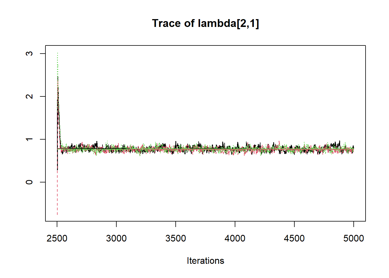
## lambda[2,1] 0.782 0.117 0.678 0.738 0.771 0.809 0.892 1.028 440
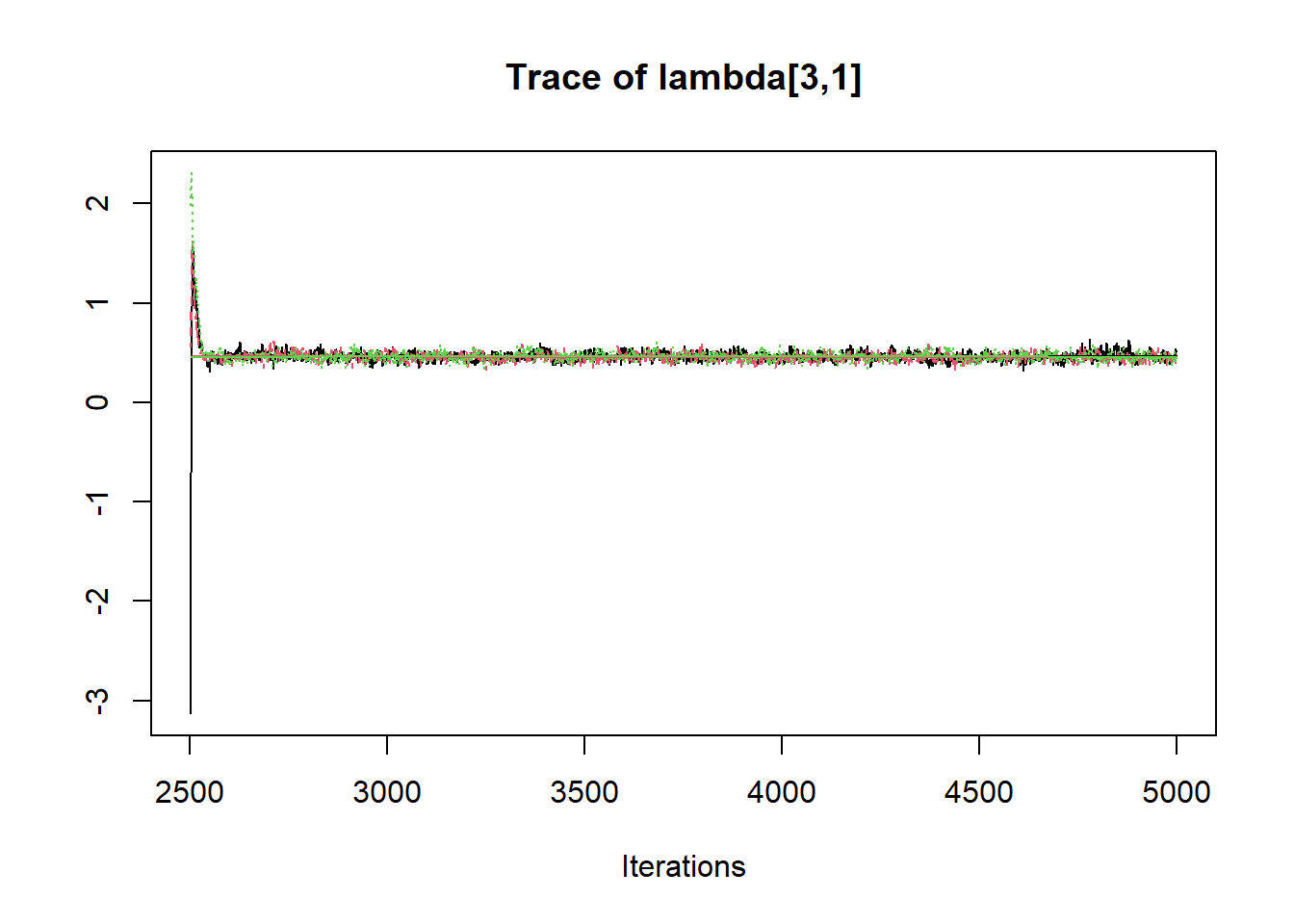
## lambda[3,1] 0.466 0.097 0.382 0.431 0.459 0.488 0.555 1.031 820
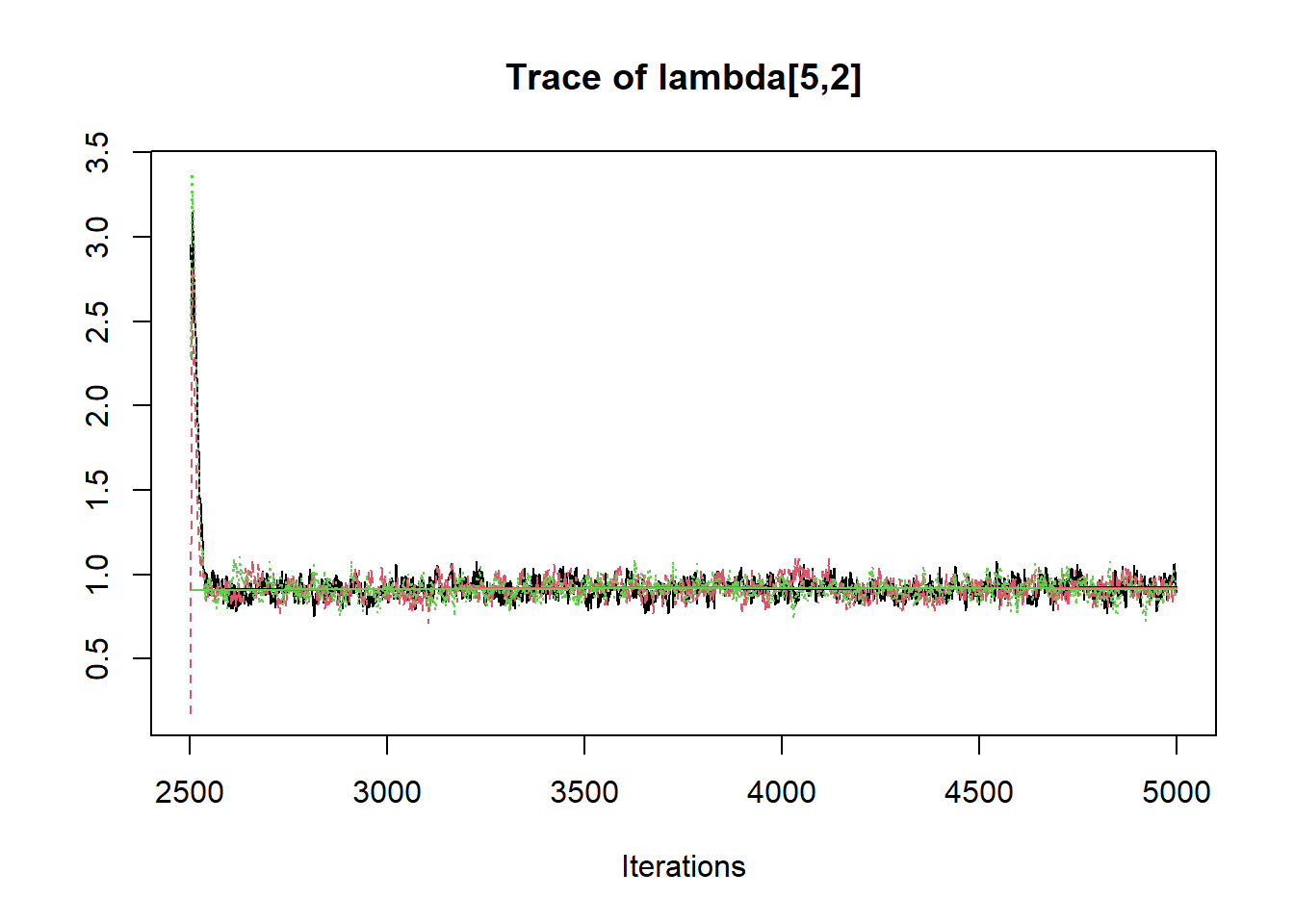
## lambda[5,2] 0.929 0.150 0.817 0.880 0.915 0.953 1.037 1.005 7500
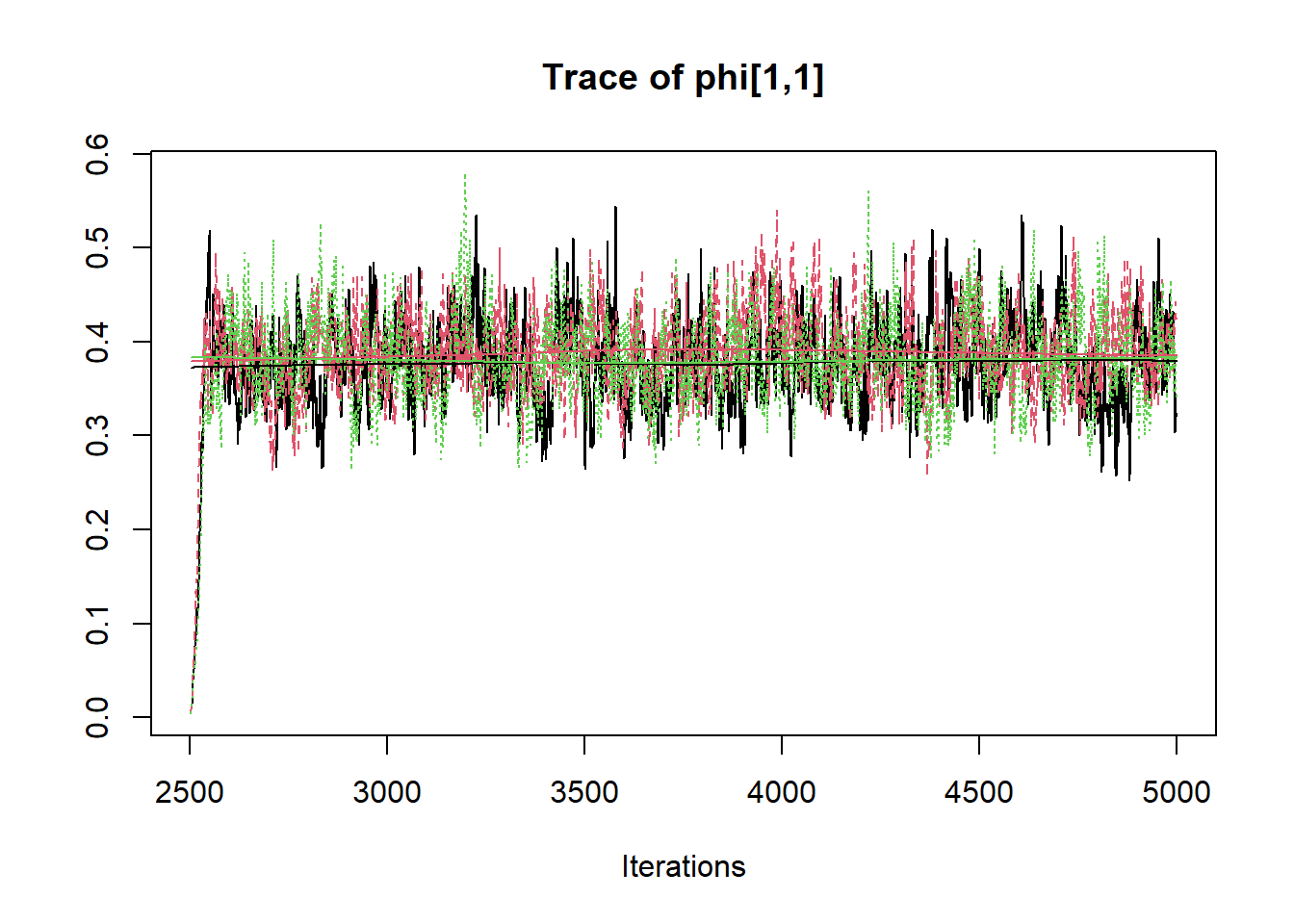
## phi[1,1] 0.380 0.053 0.293 0.351 0.381 0.411 0.472 1.005 650
## phi[2,1] 0.375 0.048 0.303 0.352 0.376 0.402 0.453 1.002 2600
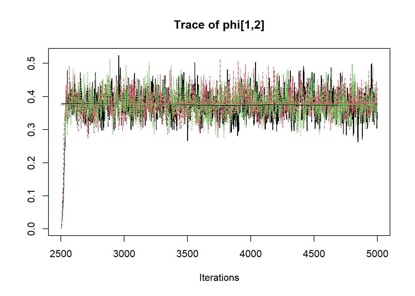
## phi[1,2] 0.375 0.048 0.303 0.352 0.376 0.402 0.453 1.002 2600
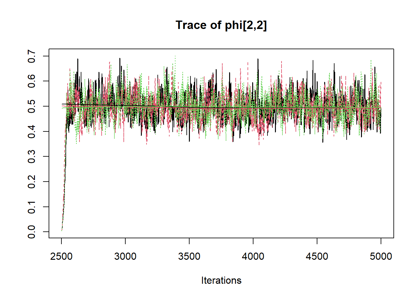
## phi[2,2] 0.493 0.066 0.393 0.461 0.495 0.531 0.602 1.001 7500
## psi[1] 0.368 0.035 0.310 0.346 0.365 0.386 0.432 1.003 850
## psi[2] 0.173 0.174 0.144 0.161 0.170 0.179 0.199 1.017 7500
## psi[3] 0.174 0.241 0.149 0.163 0.171 0.179 0.196 1.040 2100
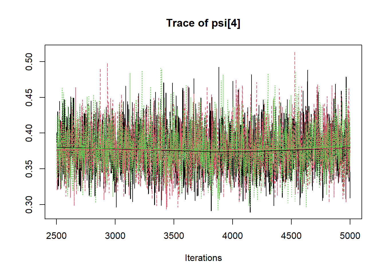
## psi[4] 0.343 0.125 0.284 0.318 0.338 0.359 0.405 1.005 7500
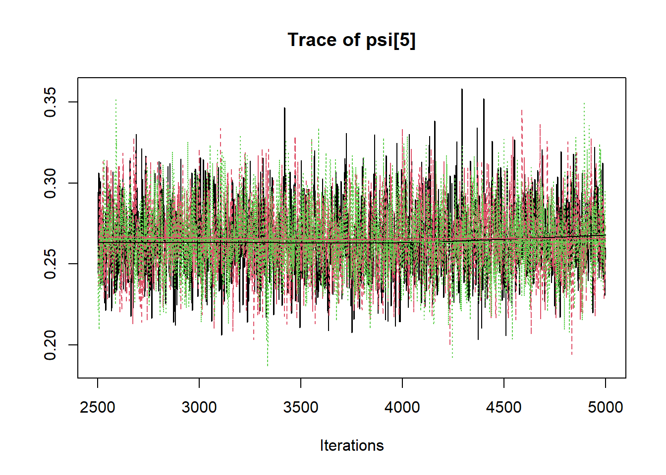
## psi[5] 0.245 0.141 0.204 0.228 0.242 0.257 0.288 1.006 7500
## tau[1] 3.334 0.038 3.260 3.308 3.334 3.360 3.410 1.001 7500
## tau[2] 3.898 0.028 3.843 3.879 3.898 3.917 3.953 1.001 7500
## tau[3] 4.596 0.023 4.551 4.581 4.596 4.611 4.640 1.001 7500
## tau[4] 3.034 0.041 2.955 3.007 3.034 3.062 3.115 1.001 7500
## tau[5] 3.713 0.036 3.641 3.689 3.713 3.738 3.784 1.001 7500
## deviance 3189.610 134.312 3072.986 3145.423 3182.566 3223.278 3306.219 1.011 7500
##
## For each parameter, n.eff is a crude measure of effective sample size,
## and Rhat is the potential scale reduction factor (at convergence, Rhat=1).
##
## DIC info (using the rule, pD = var(deviance)/2)
## pD = 9022.3 and DIC = 12211.9
## DIC is an estimate of expected predictive error (lower deviance is better).
# extract posteriors for all chains
jags.mcmc <- as.mcmc(fit)
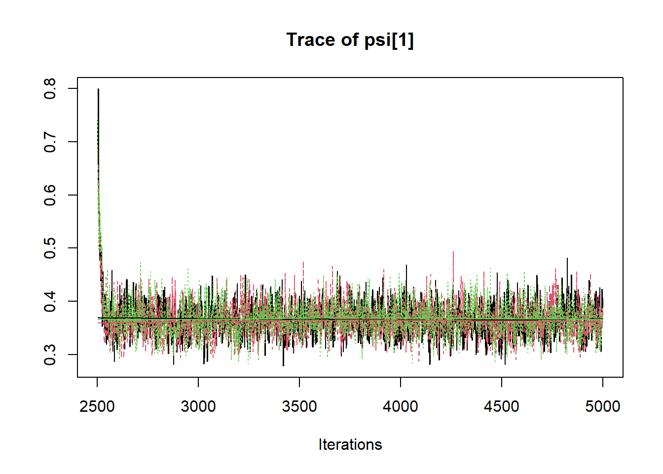
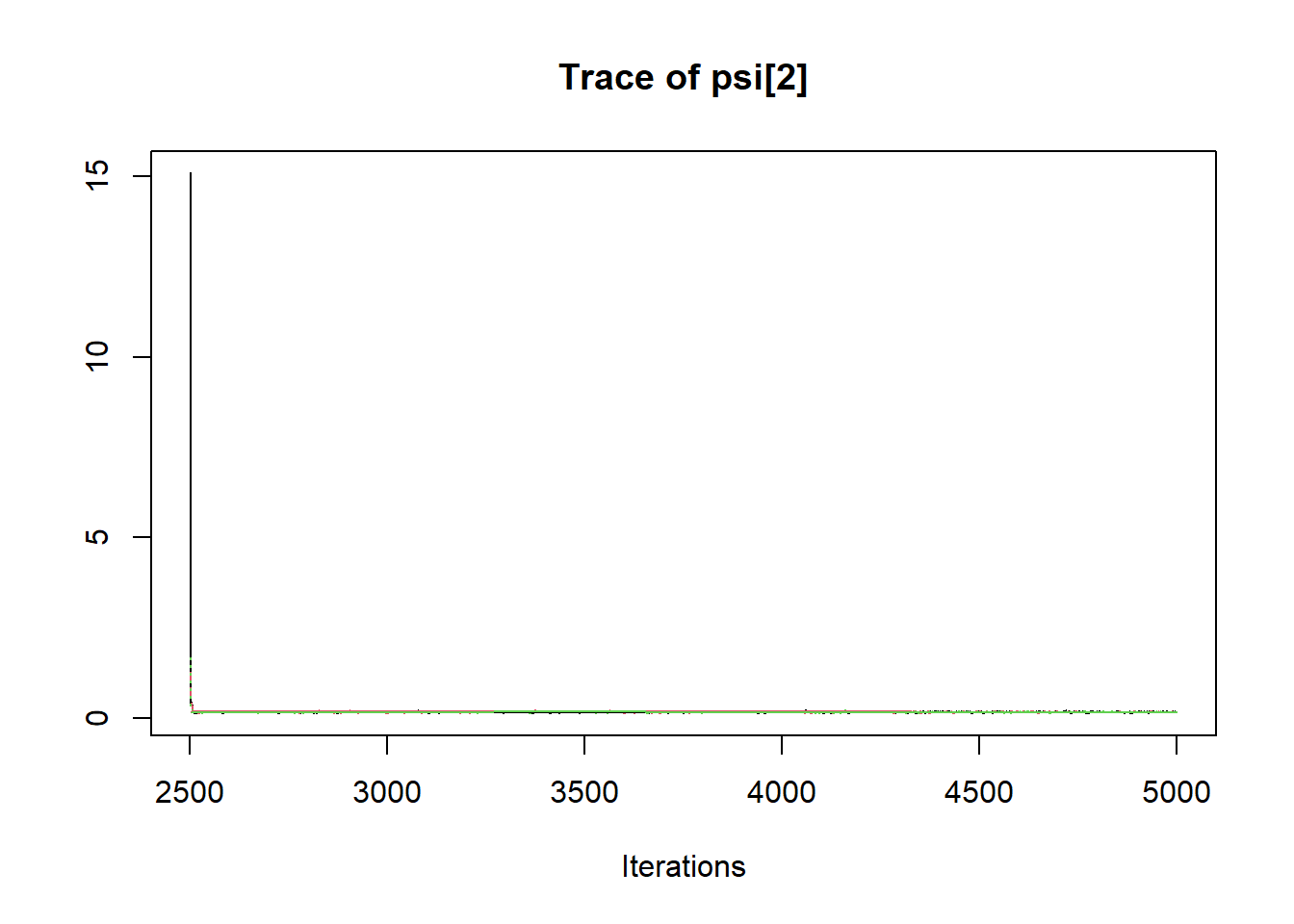
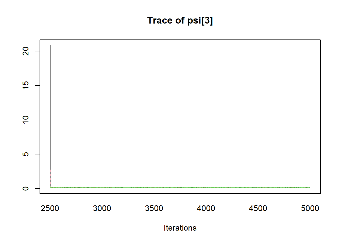
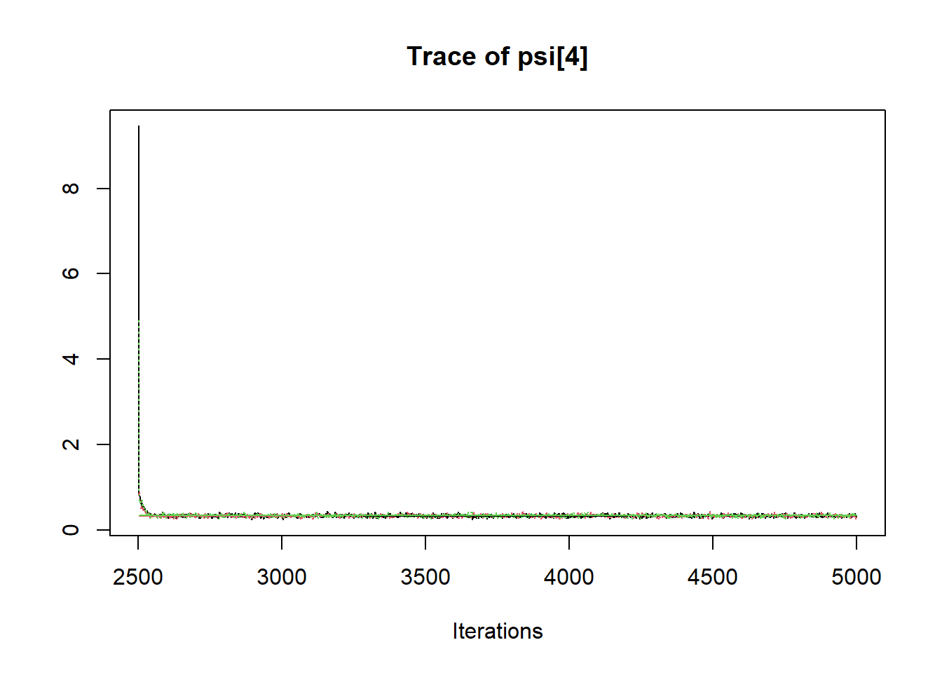
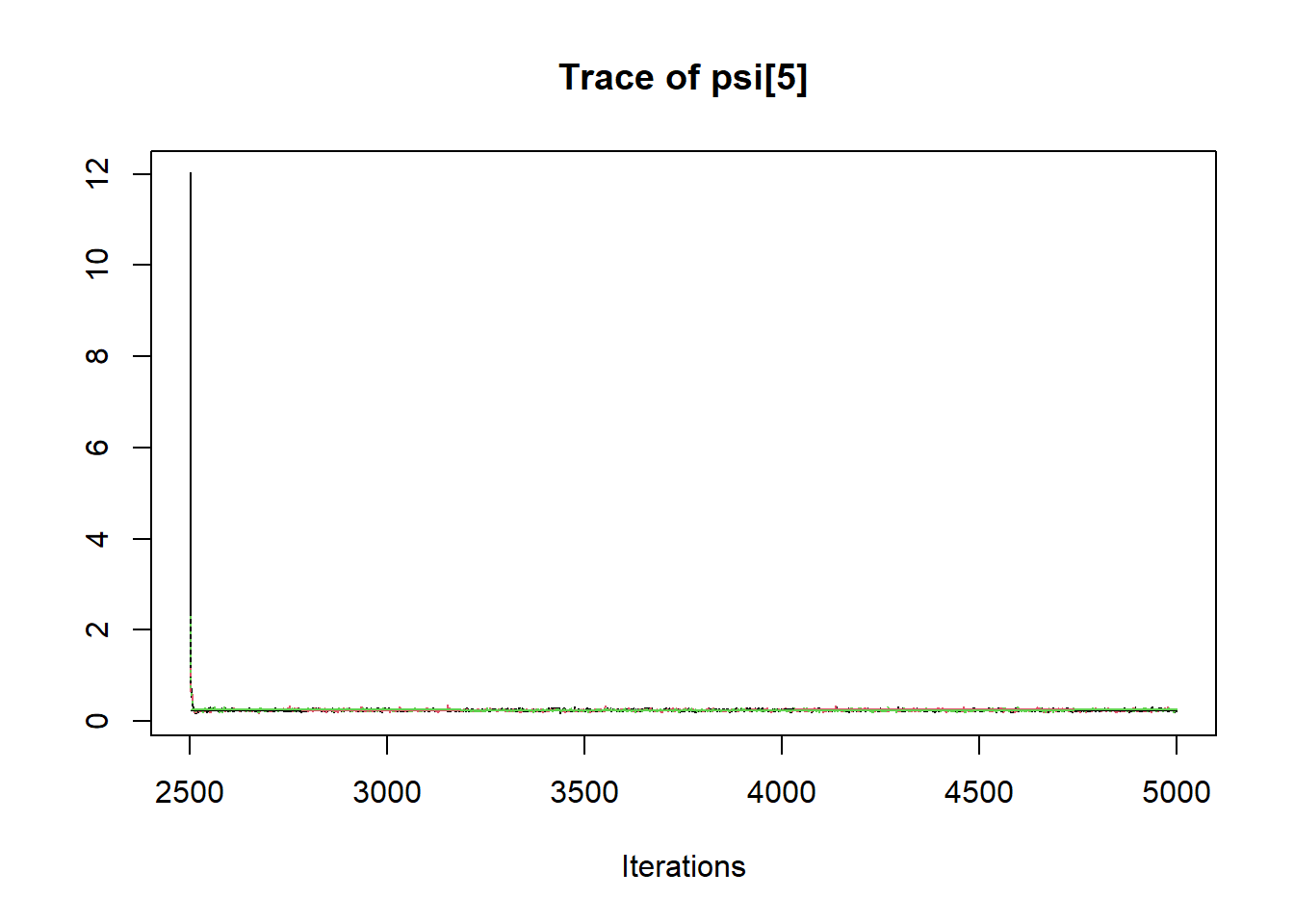
R2jags::traceplot(jags.mcmc)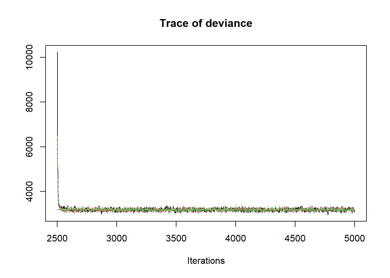

# gelman-rubin-brook
gelman.plot(jags.mcmc)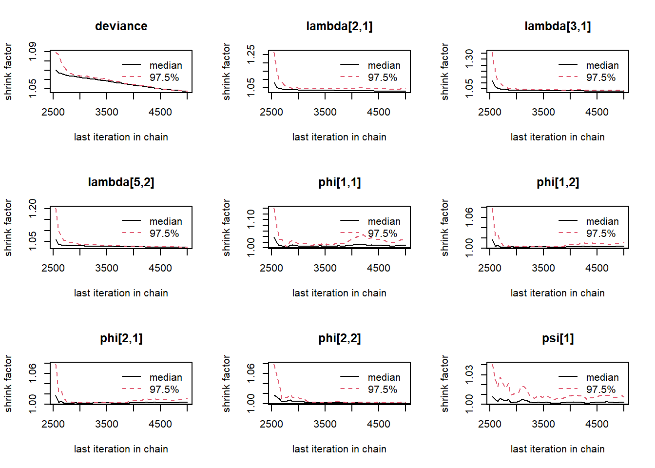
# convert to single data.frame for density plot
a <- colnames(as.data.frame(jags.mcmc[[1]]))
plot.data <- data.frame(as.matrix(jags.mcmc, chains=T, iters = T))
colnames(plot.data) <- c("chain", "iter", a)


plot_title <- ggtitle("Posterior distributions",
                      "with medians and 80% intervals")
mcmc_areas(
  plot.data,
  pars = c(paste0("tau[",1:5,"]")),
  prob = 0.8) +
  plot_title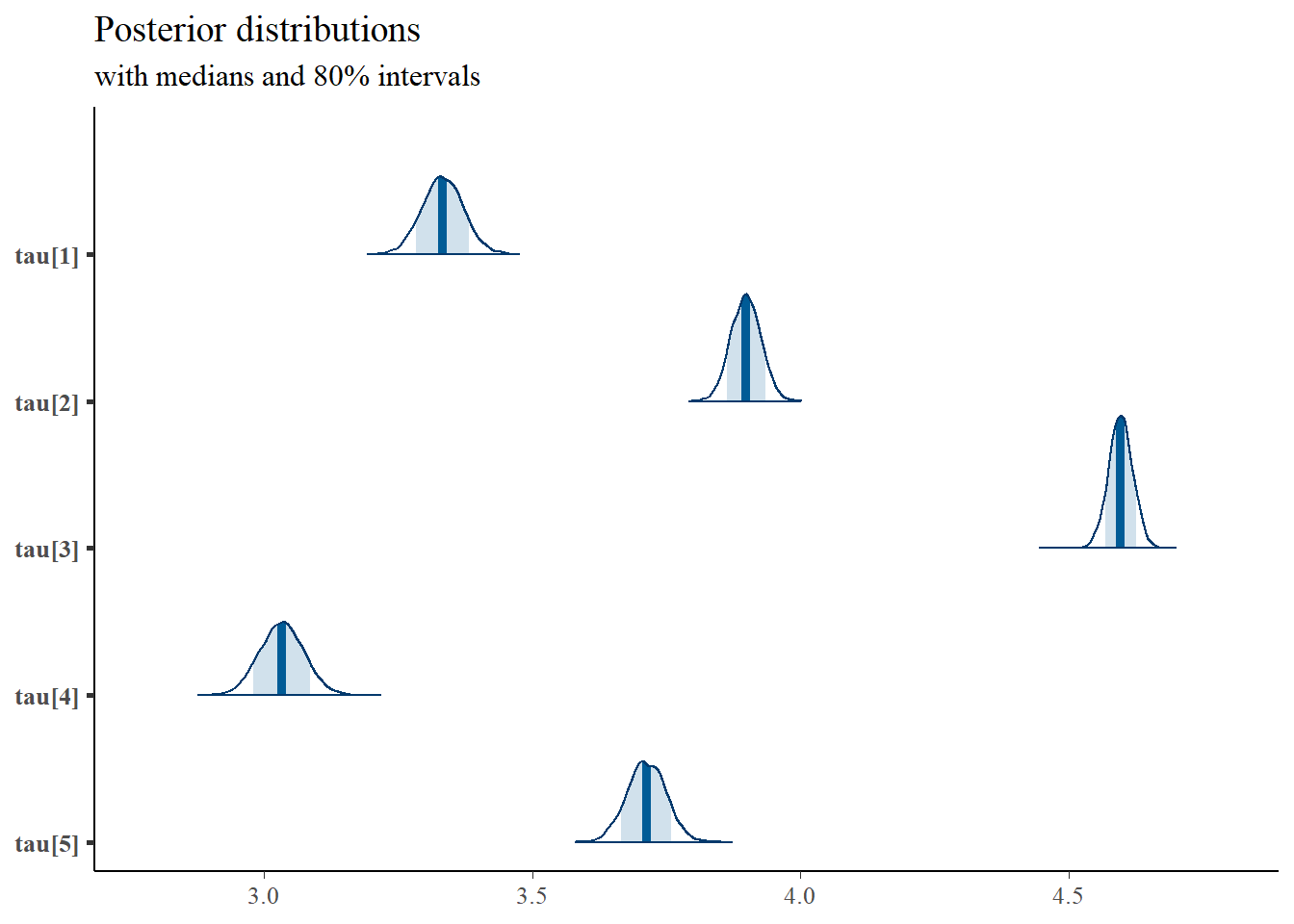
mcmc_areas(
  plot.data,
  pars = c("lambda[2,1]","lambda[3,1]","lambda[5,2]"),
  prob = 0.8) +
  plot_title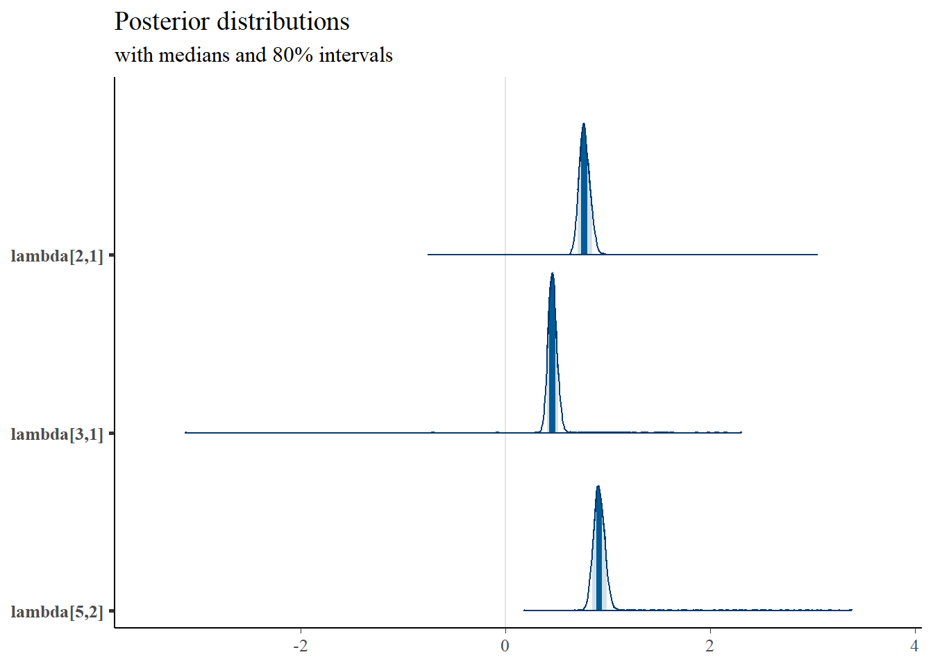
mcmc_areas(
  plot.data,
  pars = c(paste0("psi[", 1:5, "]"), "phi[1,1]", "phi[1,2]","phi[2,2]"),
  prob = 0.8) +
  plot_title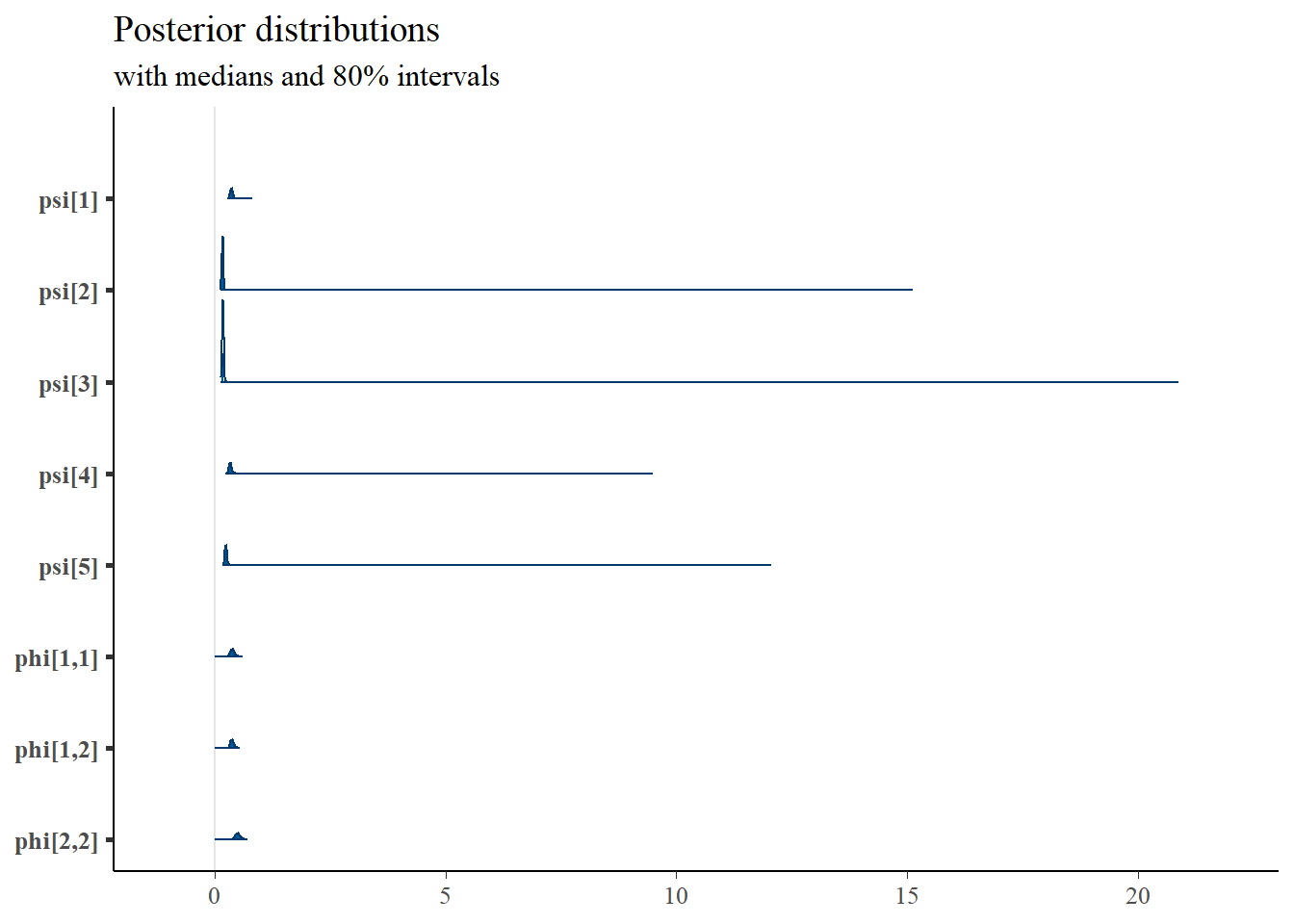
9.7 Stan - Two Latent Variable
9.7.1 Inverse-Wishart Prior
Using Stan based on a nearly identical model structure presented in the text.
model_cfa_2factor <- [1051 chars quoted with '"']

cat(model_cfa_2factor)
##
## data {
## int N;
## int J;
## int M;
## matrix[N, J] X;
## matrix[M, M] phi0;
## }
##
## parameters {
## matrix[M, M] phi; // latent variable covaraince matrix
## matrix[N, M] ksi; //latent variable values
## real lambda[J]; //factor loadings matrix
## real tau[J]; //intercepts
## real<lower=0> psi[J]; //residual variance
## }
##
## model {
## // likelihood for data
## for(i in 1:N){
## X[i, 1] ~ normal(tau[1] + ksi[i,1]*lambda[1], psi[1]);
## X[i, 2] ~ normal(tau[2] + ksi[i,1]*lambda[2], psi[2]);
## X[i, 3] ~ normal(tau[3] + ksi[i,1]*lambda[3], psi[3]);
## X[i, 4] ~ normal(tau[4] + ksi[i,2]*lambda[4], psi[4]);
## X[i, 5] ~ normal(tau[5] + ksi[i,2]*lambda[5], psi[5]);
##
## // prior for ksi
## ksi[i] ~ multi_normal(rep_vector(0, M), phi);
## }
## // latent variable variance matrix
## phi ~ inv_wishart(2, phi0);
## // prior for measurement model parameters
## tau ~ normal(3, 10);
## psi ~ inv_gamma(5, 10);
## lambda[1] ~ normal(1, .001);
## lambda[2] ~ normal(1, 10);
## lambda[3] ~ normal(1, 10);
## lambda[4] ~ normal(1, .001);
## lambda[5] ~ normal(1, 10);
## }
# data must be in a list
dat <- as.matrix(read.table("code/CFA-Two-Latent-Variables/Data/IIS.dat", header=T))

mydata <- list(
  N = 500, J = 5,
  M = 2,
  X = dat,
  phi0 = matrix(c(1, .3, .3, 1), ncol=2)
)

# # initial values
start_values <- list(
  list(
    phi= structure(
      .Data= c(1, 0.30, 0.30, 1),
      .Dim=c(2, 2)),
    tau = c(3, 3, 3, 3, 3),
    lambda= c(1, 1, 1, 1, 1),
    psi=c(.5, .5, .5, .5, .5)
  ),
  list(
    phi= structure(
      .Data= c(1, 0, 0, 1),
      .Dim=c(2, 2)),
    tau = c(5, 5, 5, 5, 5),
    lambda= c(1, .7, .7, 1, .7),
    psi=c(2, 2, 2, 2, 2)
  ),
  list(
    phi= structure(
      .Data= c(1, 0.10, 0.10, 1),
      .Dim=c(2, 2)),
    tau = c(1, 1, 1, 1, 1),
    lambda= c(1, 1.3, 1.3, 1, 1.3),
    psi=c(1, 1, 1, 1, 1)
  )
)

# Next, need to fit the model
#   I have explicitly outlined some common parameters
fit <- stan(
  model_code = model_cfa_2factor, # model code to be compiled
  data = mydata,          # my data
  init = start_values,    # starting values
  chains=3,
  refresh = 0             # no progress shown
)
## Warning: There were 2983 divergent transitions after warmup. See
## https://mc-stan.org/misc/warnings.html#divergent-transitions-after-warmup
## to find out why this is a problem and how to eliminate them.## Warning: There were 17 transitions after warmup that exceeded the maximum treedepth. Increase max_treedepth above 10. See
## https://mc-stan.org/misc/warnings.html#maximum-treedepth-exceeded## Warning: Examine the pairs() plot to diagnose sampling problems## Warning: The largest R-hat is 3.78, indicating chains have not mixed.
## Running the chains for more iterations may help. See
## https://mc-stan.org/misc/warnings.html#r-hat## Warning: Bulk Effective Samples Size (ESS) is too low, indicating posterior means and medians may be unreliable.
## Running the chains for more iterations may help. See
## https://mc-stan.org/misc/warnings.html#bulk-ess## Warning: Tail Effective Samples Size (ESS) is too low, indicating posterior variances and tail quantiles may be unreliable.
## Running the chains for more iterations may help. See
## https://mc-stan.org/misc/warnings.html#tail-ess
# first get a basic breakdown of the posteriors
print(fit,
      pars =c("lambda", "tau", "psi",
              "phi",
              "ksi[1, 1]", "ksi[1, 2]",
              "ksi[8, 1]", "ksi[8, 2]"))
## Inference for Stan model: anon_model.
## 3 chains, each with iter=2000; warmup=1000; thin=1;
## post-warmup draws per chain=1000, total post-warmup draws=3000.
##
## mean se_mean sd 2.5% 25% 50% 75% 97.5% n_eff Rhat
## lambda[1] 1.00 0.00 0.00 1.00 1.00 1.00 1.00 1.00 2 3.43
## lambda[2] 1.00 0.20 0.24 0.70 0.70 1.00 1.30 1.30 2 688044.85
## lambda[3] 1.00 0.20 0.24 0.70 0.70 1.00 1.30 1.30 2 571252.30
## lambda[4] 1.00 0.00 0.00 1.00 1.00 1.00 1.00 1.00 2 8.82
## lambda[5] 1.00 0.20 0.24 0.70 0.70 1.00 1.30 1.30 2 828681.14
## tau[1] 3.00 1.33 1.63 1.00 1.00 3.00 5.00 5.00 2 6408079.17
## tau[2] 3.00 1.33 1.63 1.00 1.00 3.00 5.00 5.00 2 4018815.25
## tau[3] 3.00 1.33 1.63 1.00 1.00 3.00 5.00 5.00 2 4477733.07
## tau[4] 3.00 1.33 1.63 1.00 1.00 3.00 5.00 5.00 2 5380093.58
## tau[5] 3.00 1.33 1.63 1.00 1.00 3.00 5.00 5.00 2 2626323.63
## psi[1] 1.17 0.51 0.62 0.50 0.50 1.00 2.00 2.00 2 1360074.81
## psi[2] 1.17 0.51 0.62 0.50 0.50 1.00 2.00 2.00 2 1250198.67
## psi[3] 1.17 0.51 0.62 0.50 0.50 1.00 2.00 2.00 2 1082592.54
## psi[4] 1.17 0.51 0.62 0.50 0.50 1.00 2.00 2.00 2 1498131.27
## psi[5] 1.17 0.51 0.62 0.50 0.50 1.00 2.00 2.00 2 1034527.28
## phi[1,1] 1.00 0.00 0.00 1.00 1.00 1.00 1.00 1.00 3 1.55
## phi[1,2] 0.13 0.10 0.12 0.00 0.00 0.10 0.30 0.30 2 388039.24
## phi[2,1] 0.13 0.10 0.12 0.00 0.00 0.10 0.30 0.30 2 387623.00
## phi[2,2] 1.00 0.00 0.00 1.00 1.00 1.00 1.00 1.00 2 9.66
## ksi[1,1] 0.59 0.50 0.62 -0.28 -0.28 0.95 1.10 1.10 2 2255396.84
## ksi[1,2] -0.33 0.89 1.08 -1.84 -1.84 0.18 0.66 0.66 2 3056164.29
## ksi[8,1] 0.13 0.69 0.85 -0.91 -0.91 0.12 1.18 1.18 2 2760193.16
## ksi[8,2] 0.40 0.34 0.41 -0.10 -0.10 0.39 0.91 0.91 2 571386.66
##
## Samples were drawn using NUTS(diag_e) at Mon Jun 20 03:45:25 2022.
## For each parameter, n_eff is a crude measure of effective sample size,
## and Rhat is the potential scale reduction factor on split chains (at
## convergence, Rhat=1).
# plot the posterior in a
#  95% probability interval
#  and 80% to contrast the dispersion
plot(fit,
     pars =c("lambda", "tau", "psi",
              "phi",
              "ksi[1, 1]", "ksi[1, 2]",
              "ksi[8, 1]", "ksi[8, 2]"))
## ci_level: 0.8 (80% intervals)## outer_level: 0.95 (95% intervals)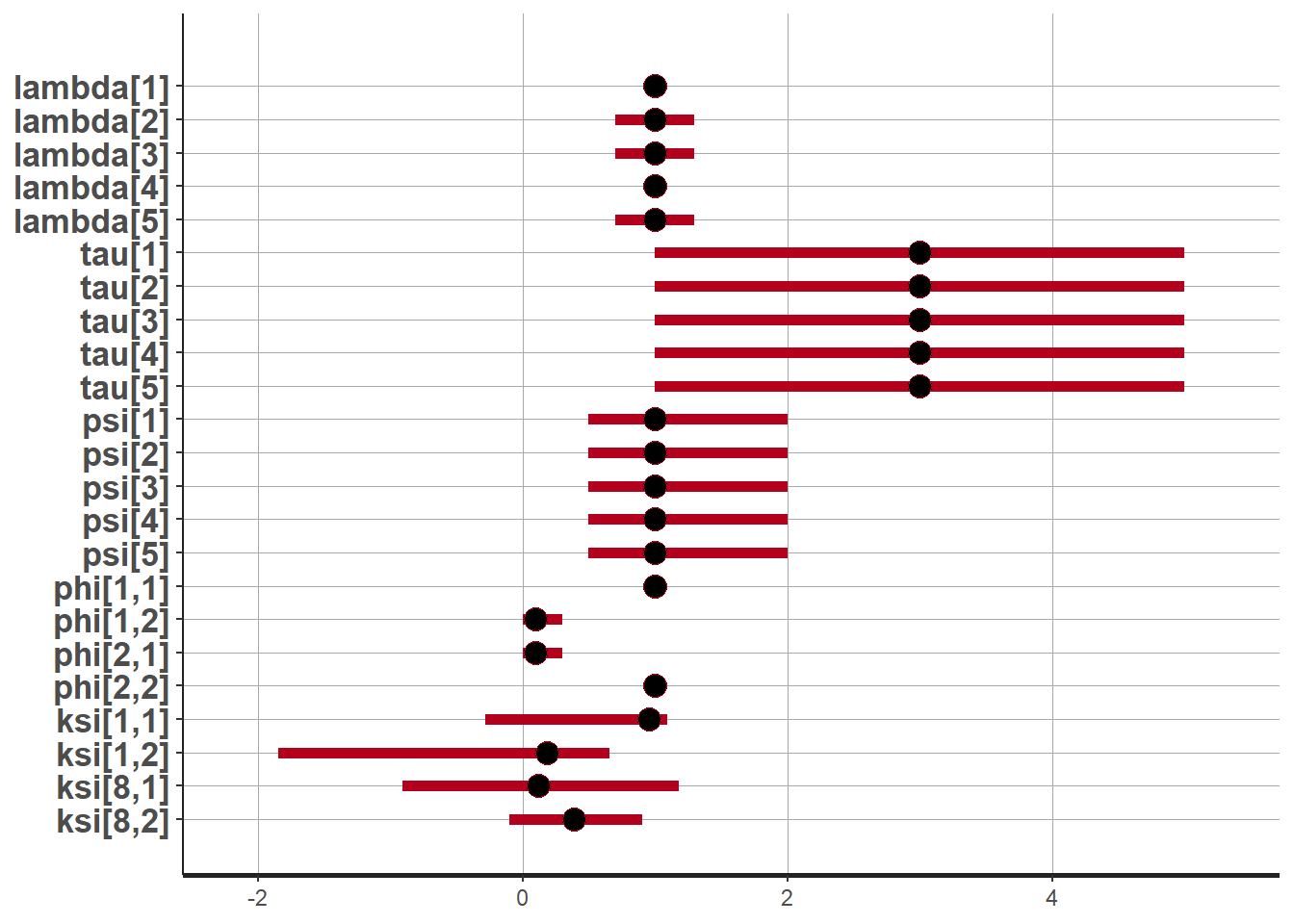
# traceplots
rstan::traceplot(
  fit,
  pars =c("lambda", "tau", "psi",
              "phi",
              "ksi[1, 1]", "ksi[1, 2]",
              "ksi[8, 1]", "ksi[8, 2]"),
  inc_warmup = TRUE)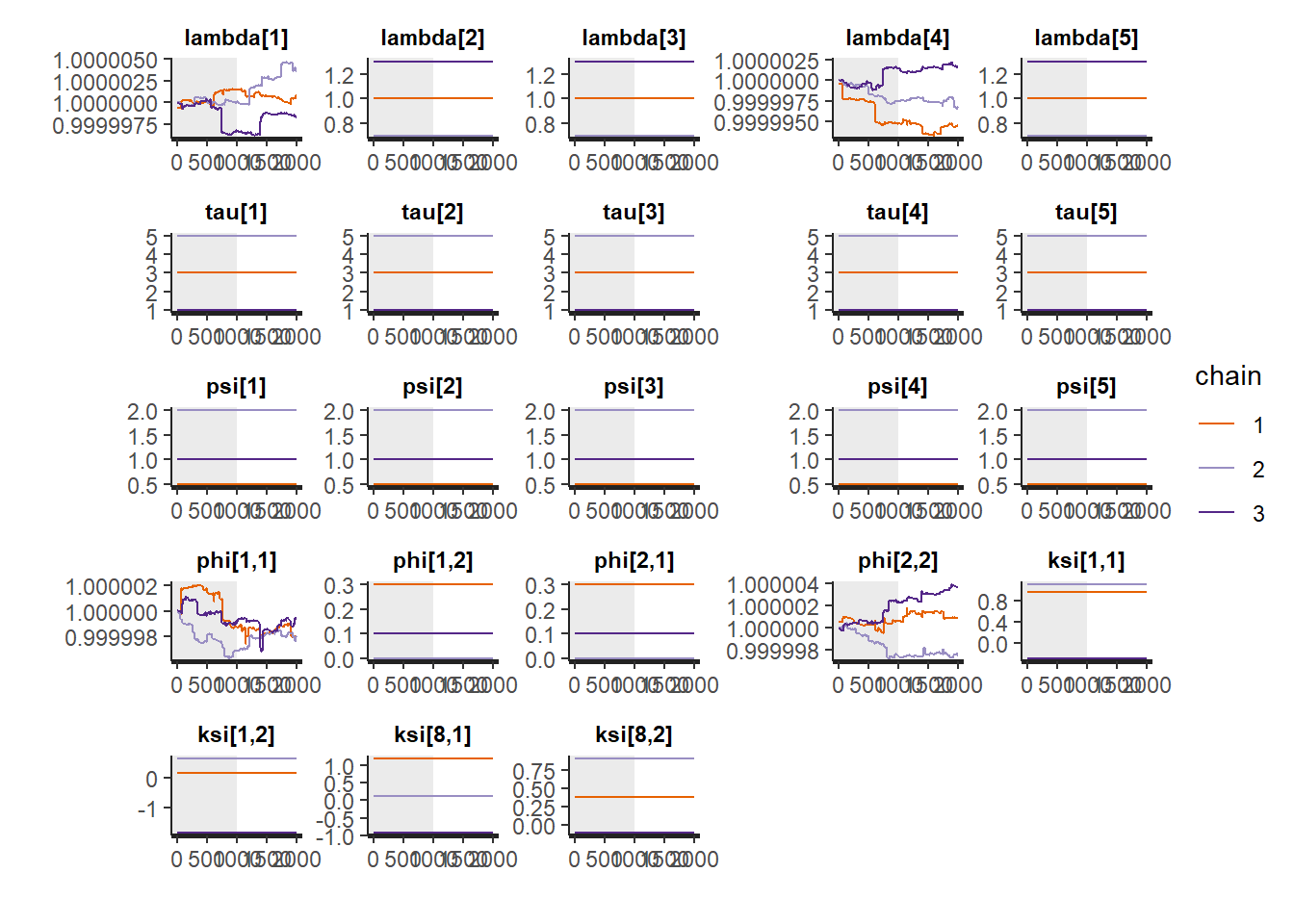
# Gelman-Rubin-Brooks Convergence Criterion
ggs_grb(ggs(fit, family = c("lambda"))) +
   theme_bw() + theme(panel.grid = element_blank())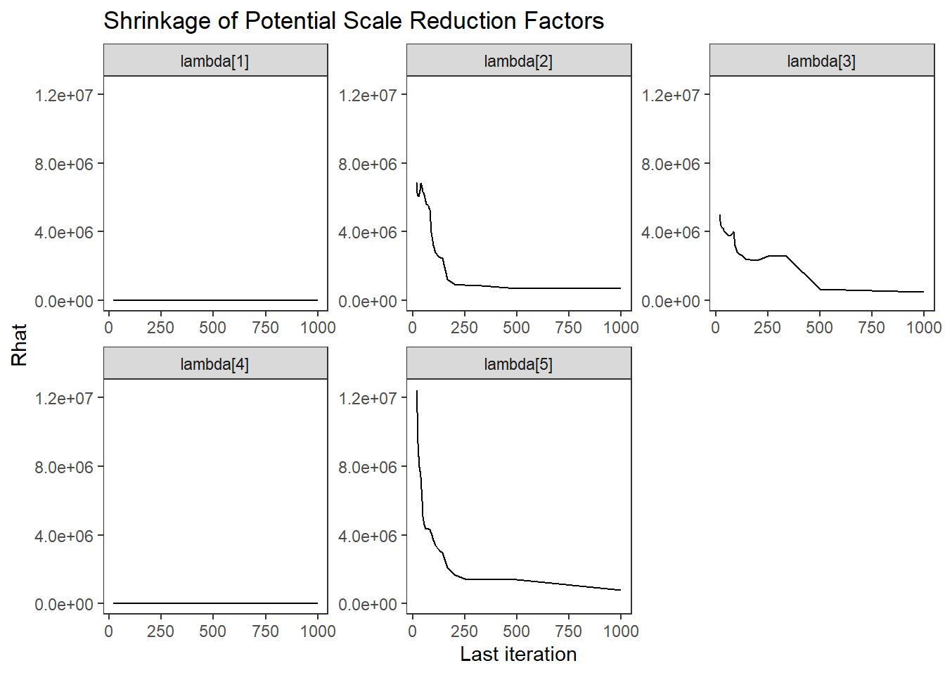
ggs_grb(ggs(fit, family = "tau")) +
   theme_bw() + theme(panel.grid = element_blank())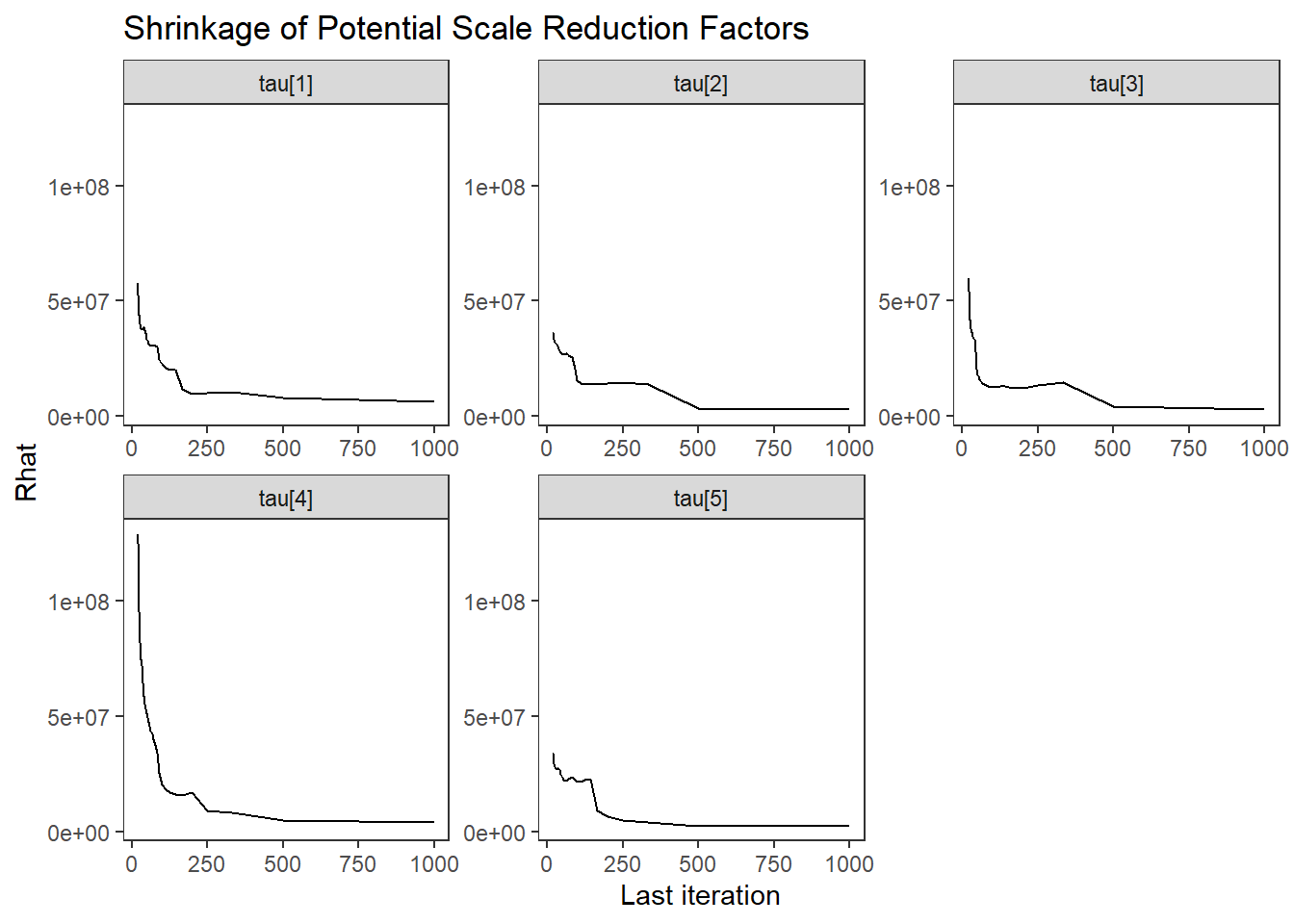
ggs_grb(ggs(fit, family = "psi")) +
   theme_bw() + theme(panel.grid = element_blank())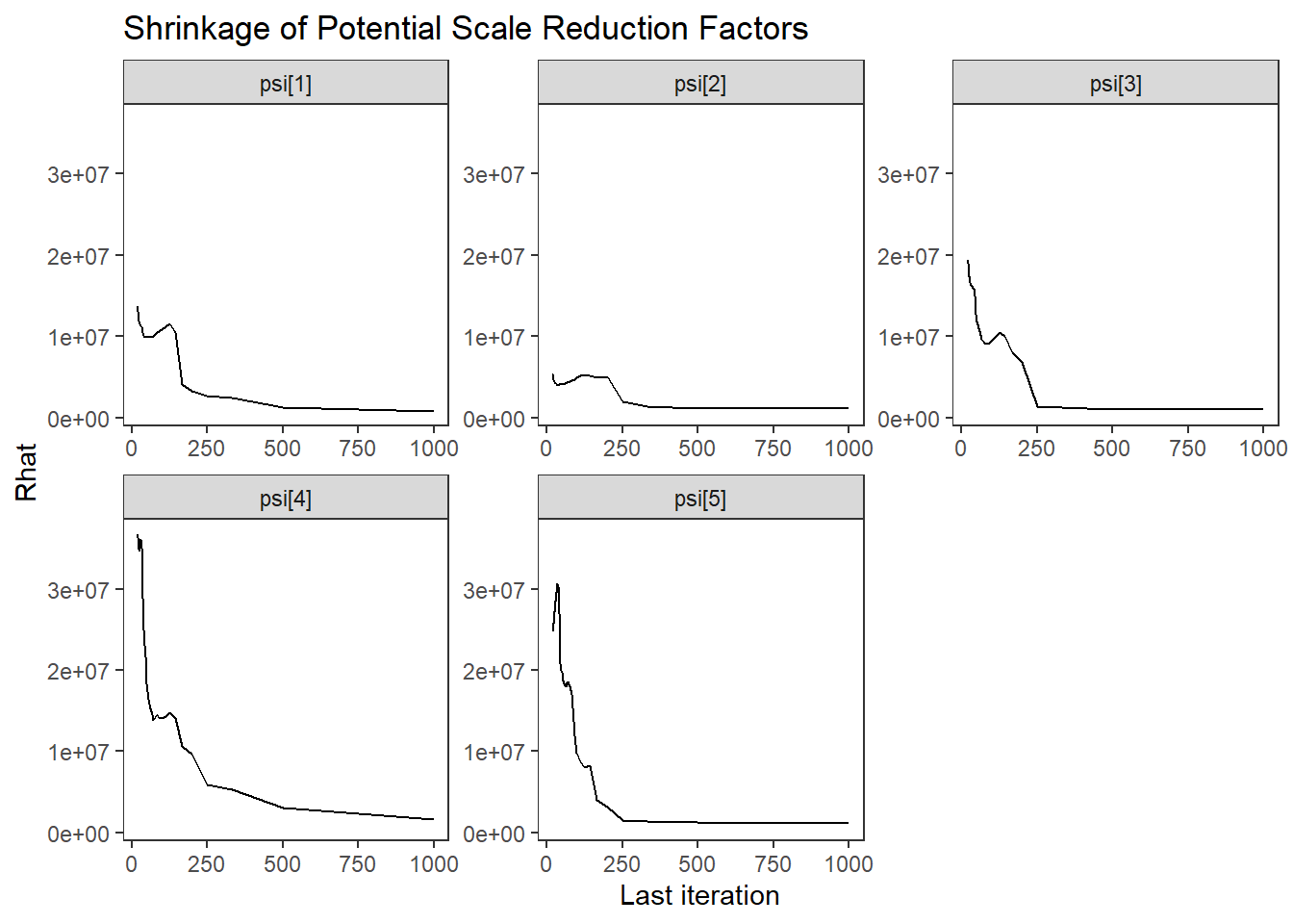
ggs_grb(ggs(fit, family = "phi")) +
   theme_bw() + theme(panel.grid = element_blank())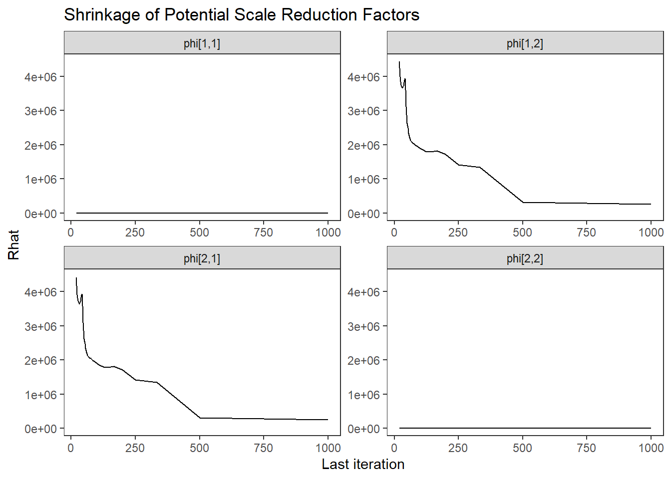
# autocorrelation
ggs_autocorrelation(ggs(fit, family="lambda")) +
   theme_bw() + theme(panel.grid = element_blank())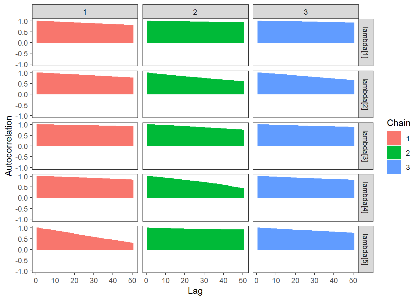
ggs_autocorrelation(ggs(fit, family="tau")) +
   theme_bw() + theme(panel.grid = element_blank())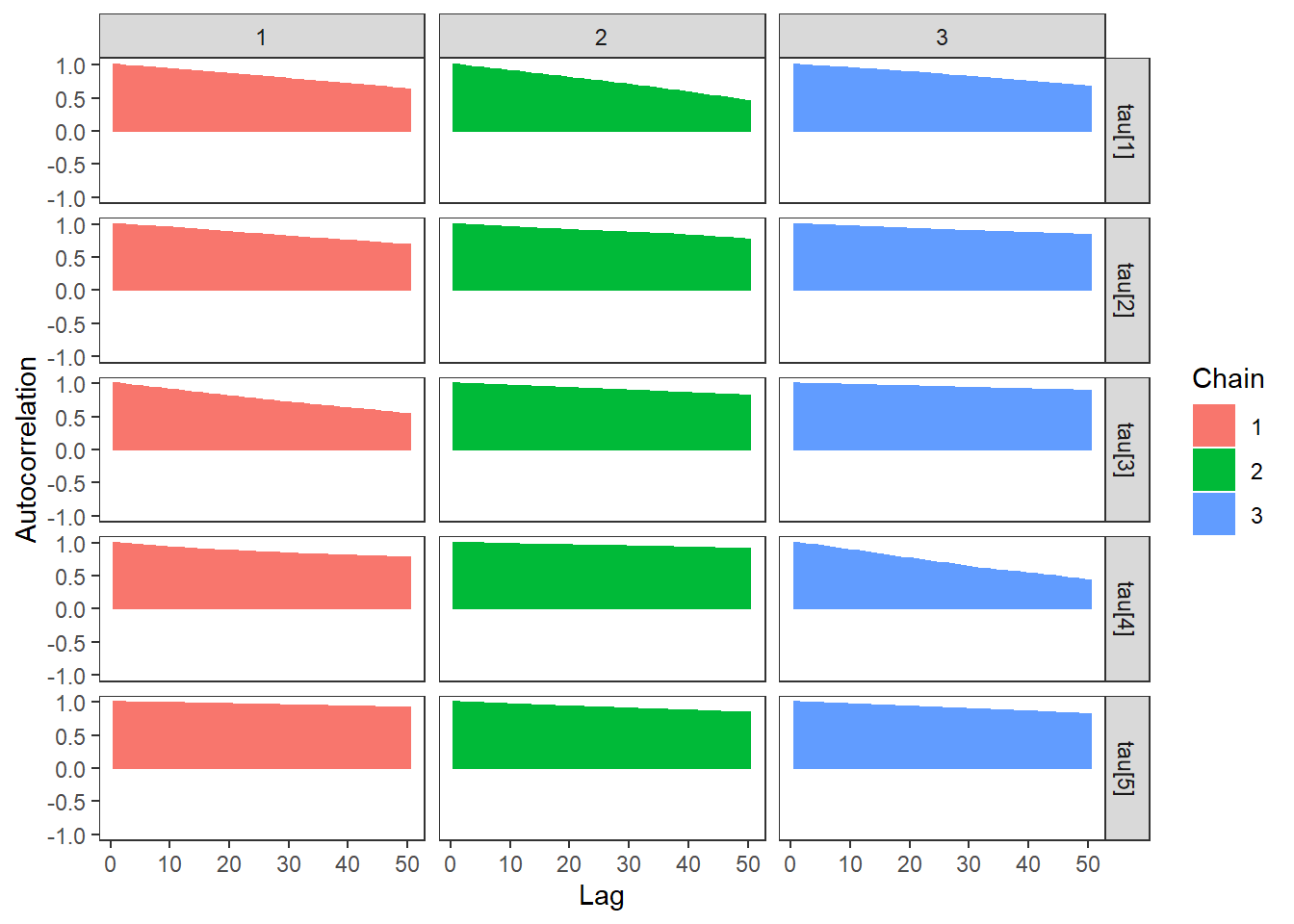
ggs_autocorrelation(ggs(fit, family="psi")) +
   theme_bw() + theme(panel.grid = element_blank())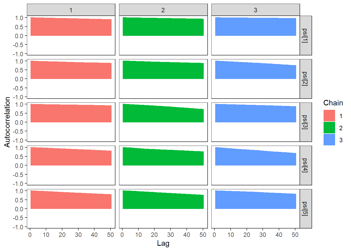
ggs_autocorrelation(ggs(fit, family="phi")) +
   theme_bw() + theme(panel.grid = element_blank())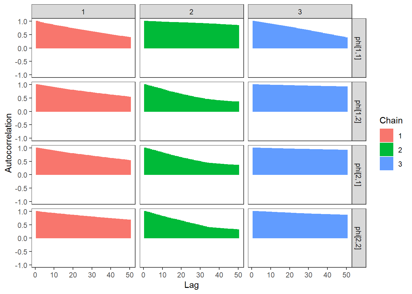
9.7.2 LKJ Cholesky Parameterization
Because I had such massive problems with the above, I search for how people estimate CFA models in Stan. I found that most people use the LKJ Cholesky parameterization.
Some helpful pages that I used to help get this to work.
- Stan User’s Guide on Factor Covaraince Parameterization
- Michael DeWitt - Confirmatory Factor Analysis in Stan
- Rick Farouni - Fitting a Bayesian Factor Analysis Model in Stan
model_cfa2 <- [1409 chars quoted with '"']

cat(model_cfa2)
##
## data {
## int N;
## int J;
## int M;
## matrix[N, J] X;
## }
##
## parameters {
## cholesky_factor_corr[M] L; // Cholesky decomp of
## // corr mat of random slopes
## vector[M] A; // Vector of factor variances
## matrix[N, M] ksi; //latent variable values
## vector[J] lambda; //factor loadings matrix
## real tau[J]; //intercepts
## real<lower=0> psi[J]; //residual variance
## }
##
## transformed parameters {
## matrix[M, M] A0;
## vector[M] S;
## A0 = diag_pre_multiply(A, L);
## S = sqrt(A);
## }
##
## model {
##
## // likelihood for data
## for(i in 1:N){
## X[i, 1] ~ normal(tau[1] + ksi[i,1]*lambda[1], psi[1]);
## X[i, 2] ~ normal(tau[2] + ksi[i,1]*lambda[2], psi[2]);
## X[i, 3] ~ normal(tau[3] + ksi[i,1]*lambda[3], psi[3]);
## X[i, 4] ~ normal(tau[4] + ksi[i,2]*lambda[4], psi[4]);
## X[i, 5] ~ normal(tau[5] + ksi[i,2]*lambda[5], psi[5]);
## }
## // latent variable parameters
## A ~ inv_gamma(5, 10);
## L ~ lkj_corr_cholesky(M);
## for(i in 1:N){
## ksi[i] ~ multi_normal_cholesky(rep_vector(0, M), A0);
## }
## // prior for measurement model parameters
## tau ~ normal(3, 10);
## psi ~ inv_gamma(5, 10);
## // factor loading patterns
## lambda[1] ~ normal(1, .001);
## lambda[2] ~ normal(1, 10);
## lambda[3] ~ normal(1, 10);
## lambda[4] ~ normal(1, .001);
## lambda[5] ~ normal(1, 10);
## }
##
## generated quantities {
## matrix[M, M] R;
## matrix[M, M] phi;
##
## R = tcrossprod(L);
## phi = quad_form_diag(R, S);
## }
# data must be in a list
dat <- as.matrix(read.table("code/CFA-Two-Latent-Variables/Data/IIS.dat", header=T))

mydata <- list(
  N = 500, J = 5,
  M = 2,
  X = dat
)

# Next, need to fit the model
#   I have explicitly outlined some common parameters
fit <- stan(
  model_code = model_cfa2, # model code to be compiled
  data = mydata,          # my data
  #init = init_fun, #start_values,    # starting values
  refresh = 0             # no progress shown
)
## Warning: Bulk Effective Samples Size (ESS) is too low, indicating posterior means and medians may be unreliable.
## Running the chains for more iterations may help. See
## https://mc-stan.org/misc/warnings.html#bulk-ess
# first get a basic breakdown of the posteriors
print(fit,
      pars =c("lambda", "tau", "psi",
              "R", "A", "A0", "phi",
              "ksi[1, 1]", "ksi[1, 2]",
              "ksi[8, 1]", "ksi[8, 2]"))
## Inference for Stan model: anon_model.
## 4 chains, each with iter=2000; warmup=1000; thin=1;
## post-warmup draws per chain=1000, total post-warmup draws=4000.
##
## mean se_mean sd 2.5% 25% 50% 75% 97.5% n_eff Rhat
## lambda[1] 1.00 0 0.00 1.00 1.00 1.00 1.00 1.00 4475 1.00
## lambda[2] 0.87 0 0.06 0.76 0.83 0.87 0.91 0.98 694 1.00
## lambda[3] 0.52 0 0.04 0.44 0.49 0.52 0.54 0.60 995 1.00
## lambda[4] 1.00 0 0.00 1.00 1.00 1.00 1.00 1.00 4225 1.00
## lambda[5] 0.96 0 0.05 0.86 0.92 0.96 1.00 1.07 849 1.00
## tau[1] 3.33 0 0.04 3.25 3.31 3.33 3.36 3.40 1067 1.00
## tau[2] 3.90 0 0.03 3.84 3.88 3.90 3.91 3.95 864 1.00
## tau[3] 4.60 0 0.02 4.55 4.58 4.60 4.61 4.64 1321 1.00
## tau[4] 3.03 0 0.04 2.95 3.00 3.03 3.06 3.11 998 1.00
## tau[5] 3.71 0 0.04 3.64 3.69 3.71 3.73 3.78 887 1.00
## psi[1] 0.61 0 0.02 0.56 0.59 0.61 0.62 0.65 2275 1.00
## psi[2] 0.32 0 0.02 0.28 0.31 0.32 0.33 0.36 1143 1.00
## psi[3] 0.36 0 0.01 0.33 0.35 0.36 0.36 0.38 2890 1.00
## psi[4] 0.57 0 0.03 0.52 0.55 0.56 0.58 0.62 2336 1.00
## psi[5] 0.42 0 0.03 0.37 0.41 0.42 0.44 0.47 1238 1.00
## R[1,1] 1.00 NaN 0.00 1.00 1.00 1.00 1.00 1.00 NaN NaN
## R[1,2] 0.86 0 0.03 0.80 0.84 0.86 0.88 0.91 601 1.01
## R[2,1] 0.86 0 0.03 0.80 0.84 0.86 0.88 0.91 601 1.01
## R[2,2] 1.00 NaN 0.00 1.00 1.00 1.00 1.00 1.00 NaN NaN
## A[1] 0.60 0 0.04 0.53 0.58 0.60 0.62 0.67 840 1.00
## A[2] 0.71 0 0.04 0.64 0.68 0.71 0.73 0.78 1216 1.00
## A0[1,1] 0.60 0 0.04 0.53 0.58 0.60 0.62 0.67 840 1.00
## A0[1,2] 0.00 NaN 0.00 0.00 0.00 0.00 0.00 0.00 NaN NaN
## A0[2,1] 0.61 0 0.04 0.53 0.58 0.61 0.63 0.68 1440 1.00
## A0[2,2] 0.36 0 0.04 0.29 0.34 0.36 0.39 0.43 501 1.01
## phi[1,1] 0.60 0 0.04 0.53 0.58 0.60 0.62 0.67 840 1.00
## phi[1,2] 0.56 0 0.03 0.50 0.54 0.56 0.58 0.63 1062 1.00
## phi[2,1] 0.56 0 0.03 0.50 0.54 0.56 0.58 0.63 1062 1.00
## phi[2,2] 0.71 0 0.04 0.64 0.68 0.71 0.73 0.78 1216 1.00
## ksi[1,1] -0.22 0 0.23 -0.66 -0.38 -0.22 -0.06 0.24 6673 1.00
## ksi[1,2] -0.37 0 0.28 -0.92 -0.56 -0.36 -0.18 0.17 7072 1.00
## ksi[8,1] 0.92 0 0.24 0.46 0.75 0.92 1.07 1.39 5711 1.00
## ksi[8,2] 0.88 0 0.27 0.35 0.70 0.89 1.06 1.42 7048 1.00
##
## Samples were drawn using NUTS(diag_e) at Mon Jun 20 03:53:27 2022.
## For each parameter, n_eff is a crude measure of effective sample size,
## and Rhat is the potential scale reduction factor on split chains (at
## convergence, Rhat=1).
# plot the posterior in a
#  95% probability interval
#  and 80% to contrast the dispersion
plot(fit,pars =c("lambda", "tau", "psi",
                 "phi",
              "ksi[1, 1]", "ksi[1, 2]",
              "ksi[8, 1]", "ksi[8, 2]"))
## ci_level: 0.8 (80% intervals)## outer_level: 0.95 (95% intervals)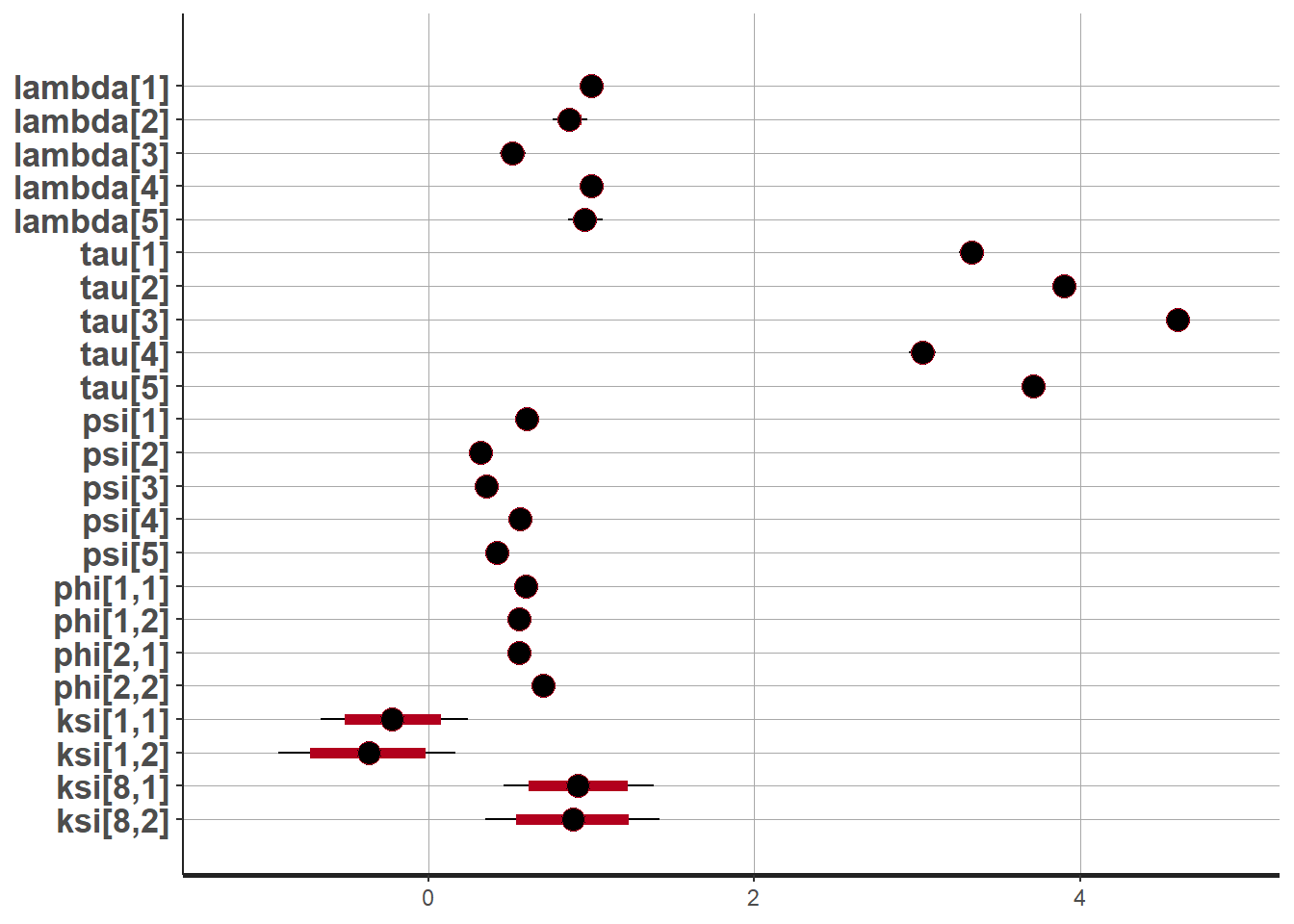
# traceplots
rstan::traceplot(fit,
      pars =c("lambda", "tau", "psi",
              "phi",
              "ksi[1, 1]", "ksi[1, 2]",
              "ksi[8, 1]", "ksi[8, 2]"), inc_warmup = TRUE)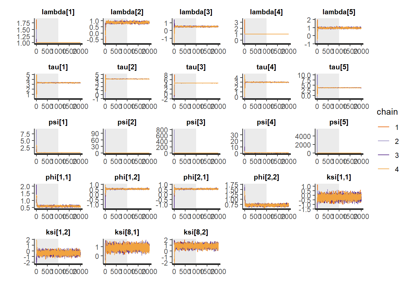
# Gelman-Rubin-Brooks Convergence Criterion
ggs_grb(ggs(fit, family = c("lambda"))) +
   theme_bw() + theme(panel.grid = element_blank())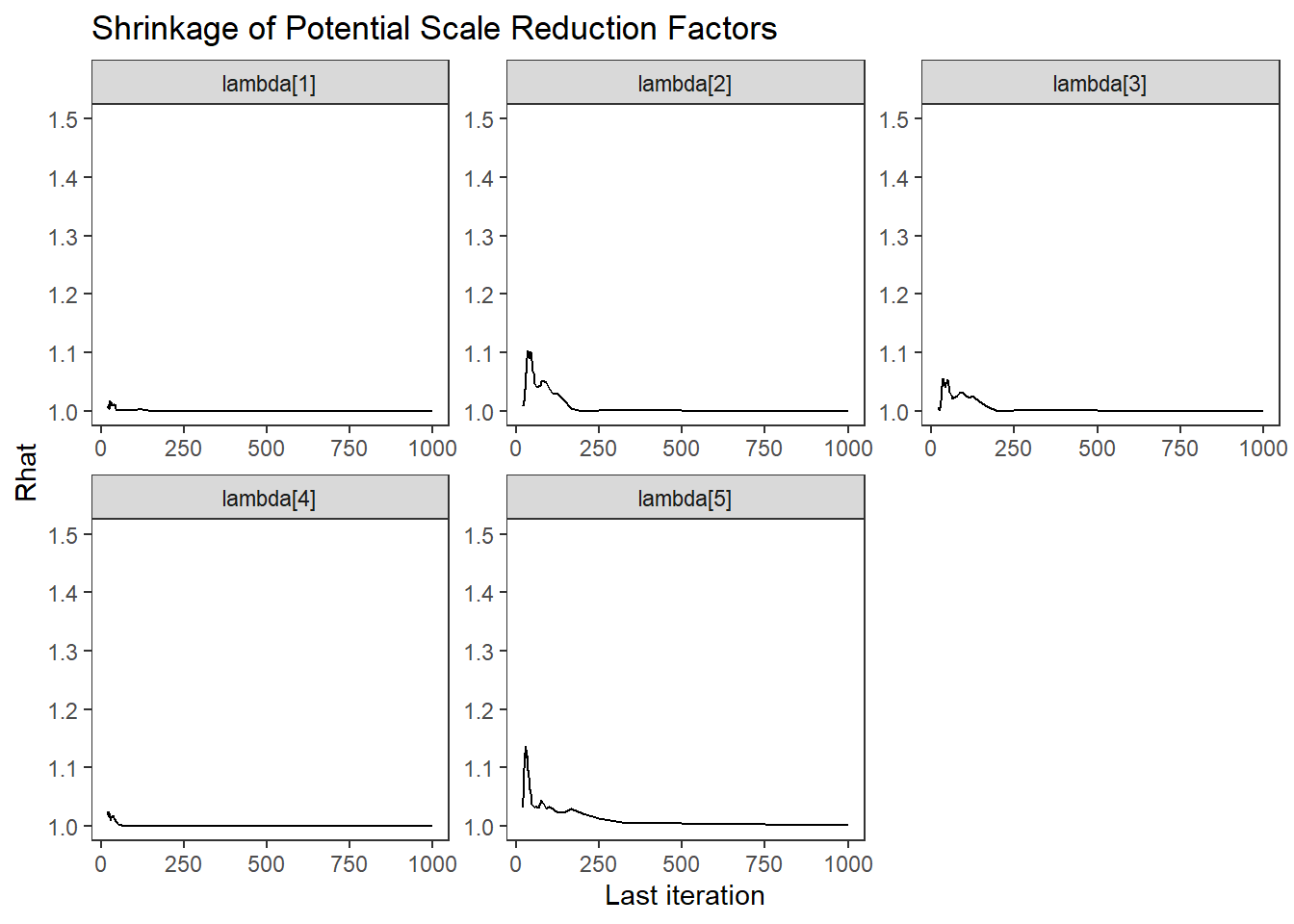
ggs_grb(ggs(fit, family = "tau")) +
   theme_bw() + theme(panel.grid = element_blank())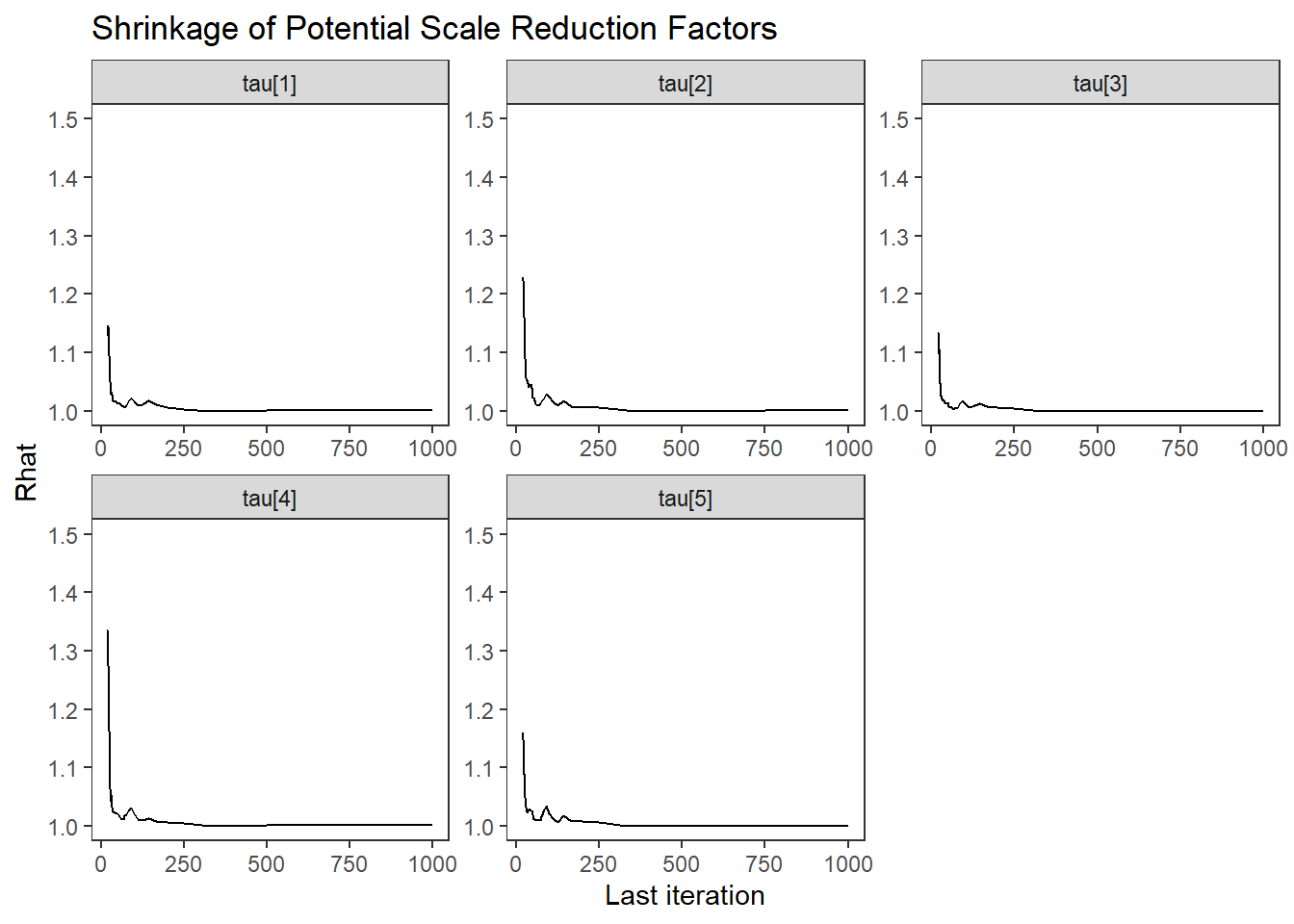
ggs_grb(ggs(fit, family = "psi")) +
   theme_bw() + theme(panel.grid = element_blank())
ggs_grb(ggs(fit, family = "phi")) +
   theme_bw() + theme(panel.grid = element_blank())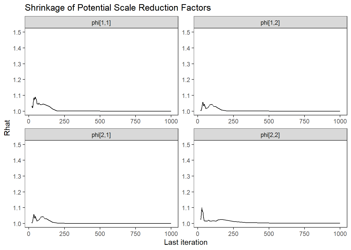
# autocorrelation
ggs_autocorrelation(ggs(fit, family="lambda")) +
   theme_bw() + theme(panel.grid = element_blank())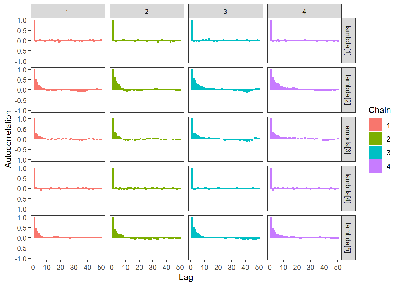
ggs_autocorrelation(ggs(fit, family="tau")) +
   theme_bw() + theme(panel.grid = element_blank())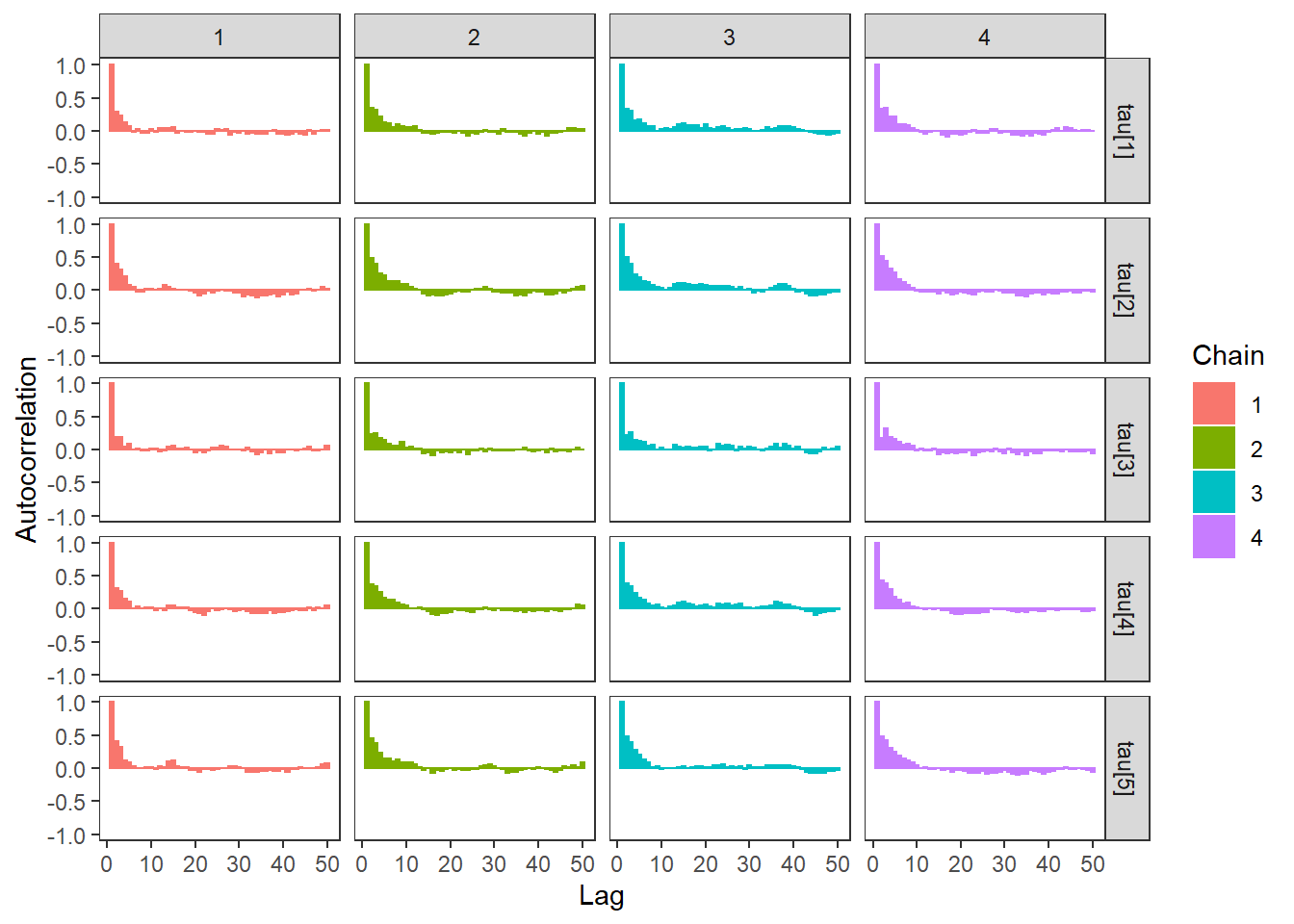
ggs_autocorrelation(ggs(fit, family="psi")) +
   theme_bw() + theme(panel.grid = element_blank())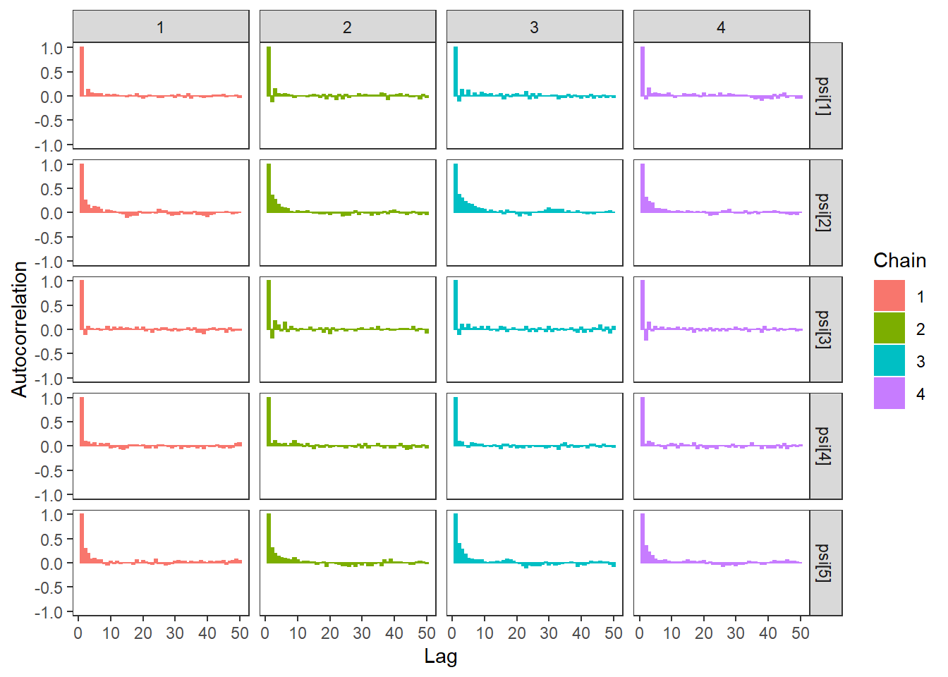
ggs_autocorrelation(ggs(fit, family="phi")) +
   theme_bw() + theme(panel.grid = element_blank())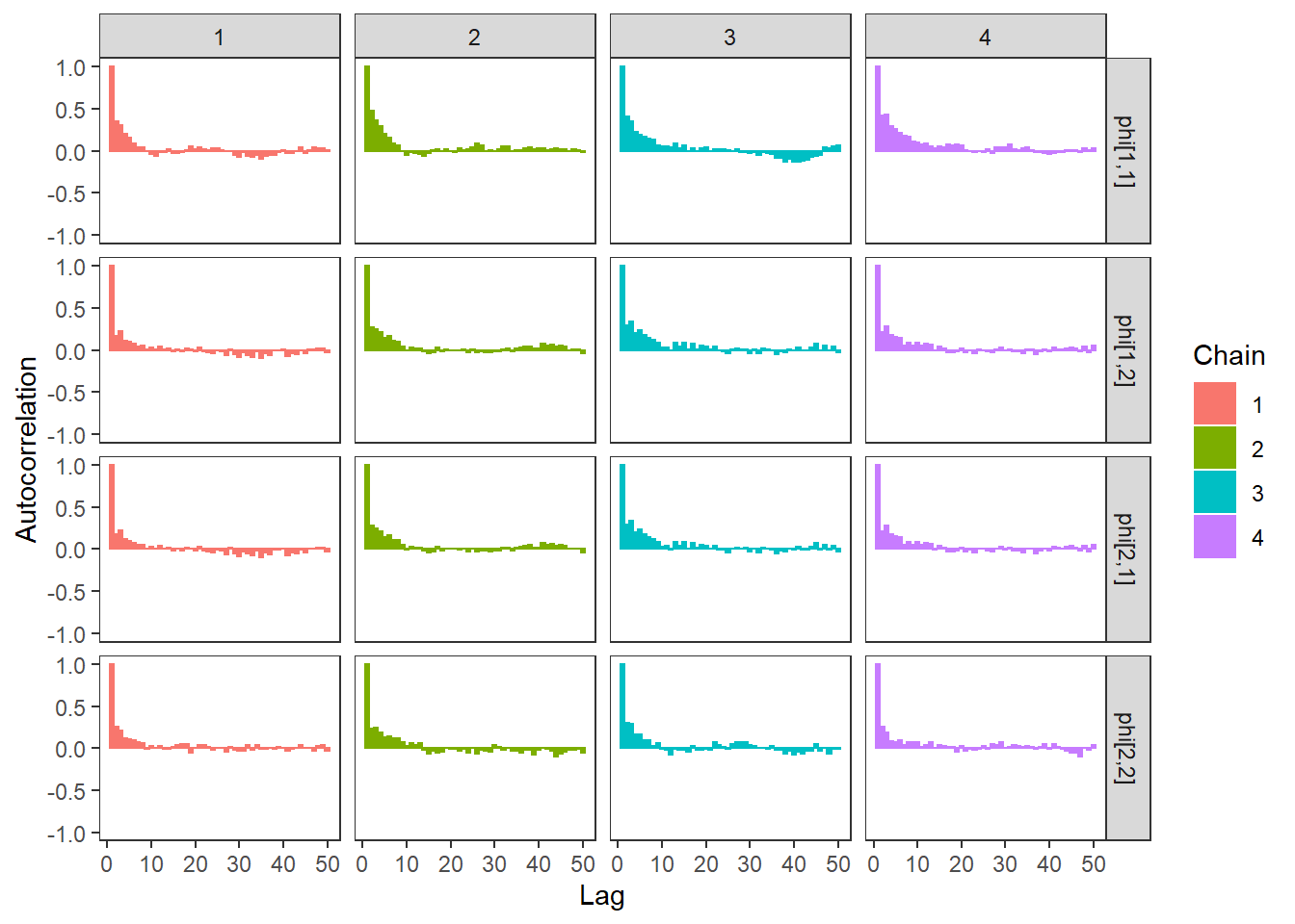
# plot the posterior density
plot.data <- as.matrix(fit)

plot_title <- ggtitle("Posterior distributions",
                      "with medians and 80% intervals")
mcmc_areas(
  plot.data,
  pars = c("lambda[2]", "lambda[3]", "lambda[5]"),
  prob = 0.8) +
  plot_title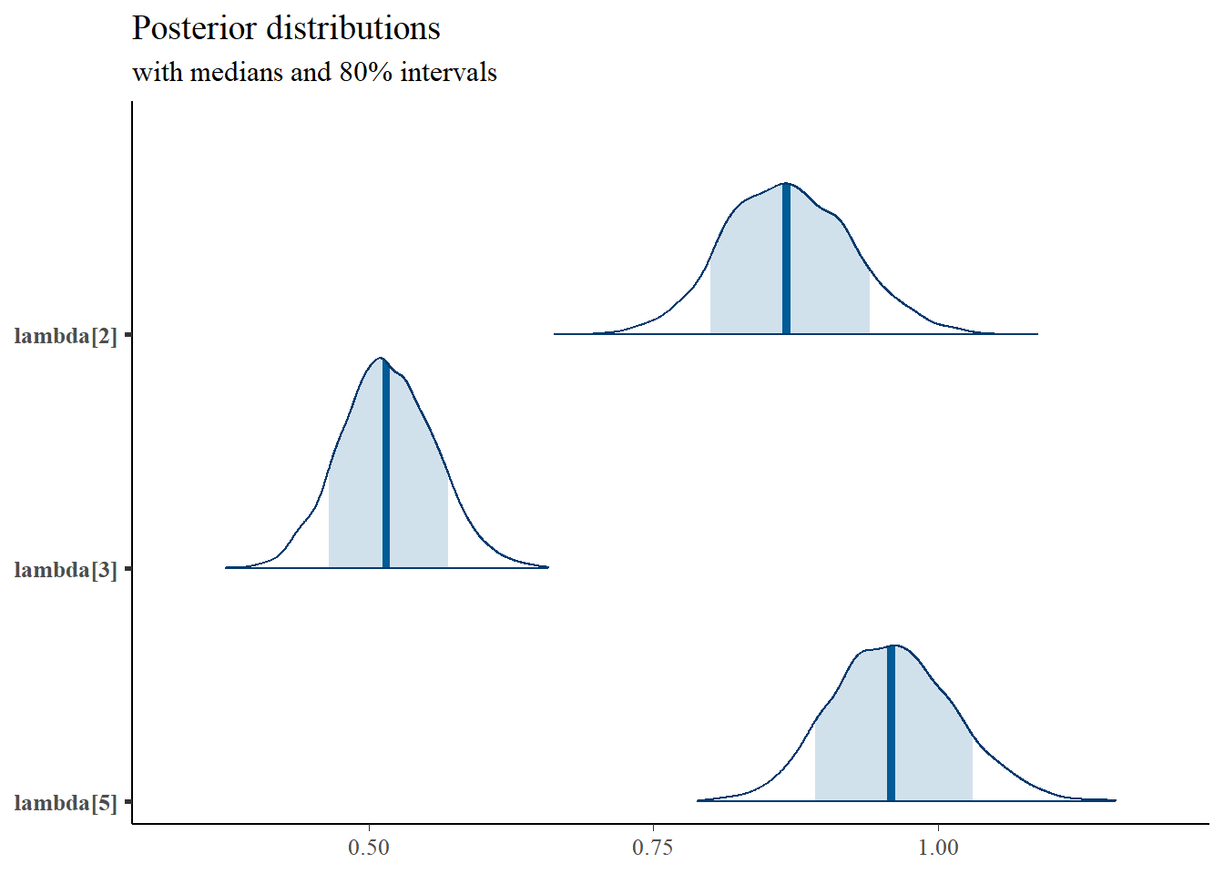
mcmc_areas(
  plot.data,
  pars = paste0("tau[",1:5,"]"),
  prob = 0.8) +
  plot_title
mcmc_areas(
  plot.data,
  pars = c(paste0("psi[",1:5,"]"),
           "phi[1,1]", "phi[1,2]", "phi[2,2]"),
  prob = 0.8) +
  plot_title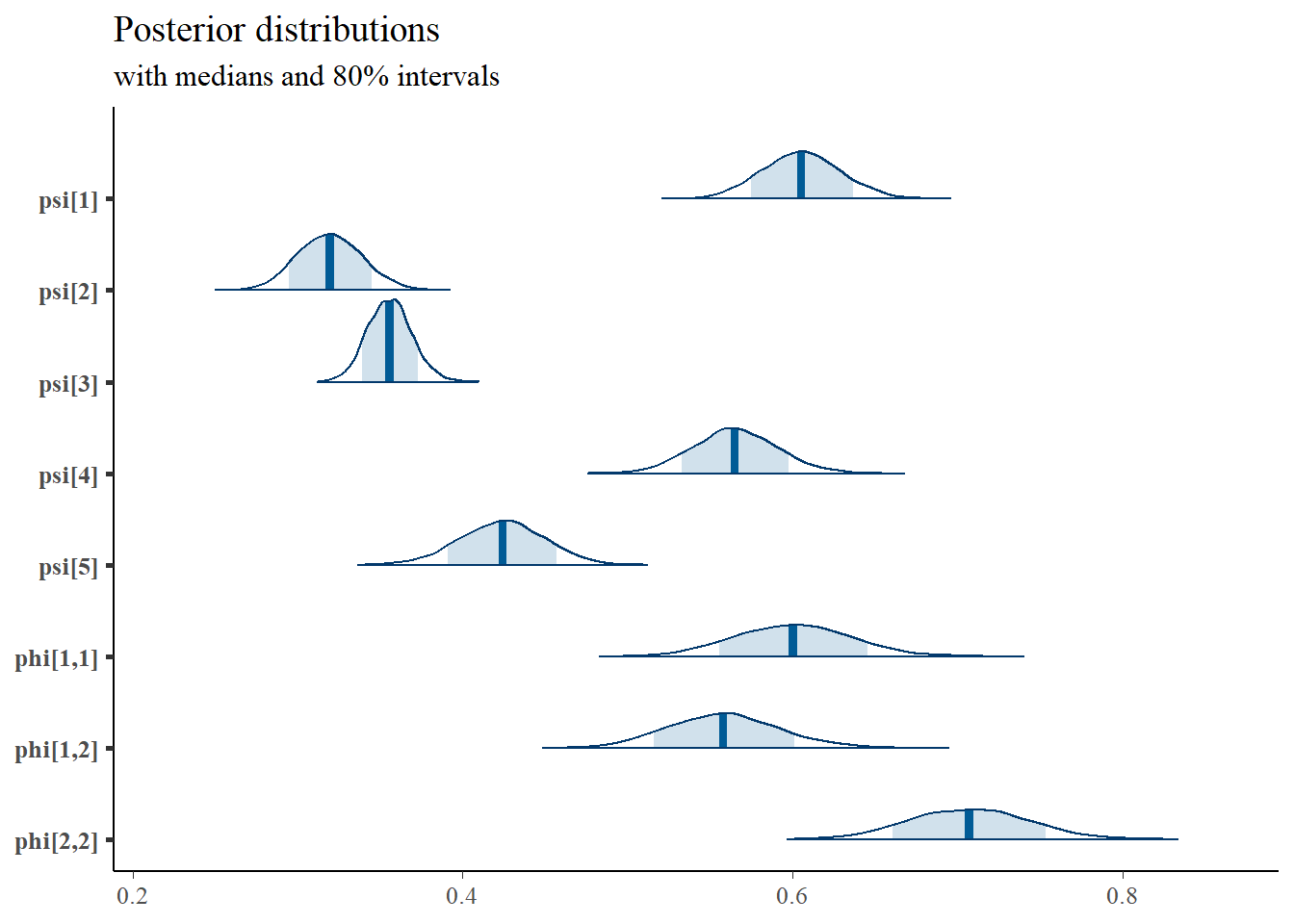
9.8 Blavaan - Two Latent Variables
# model
model_cfa2_blavaan <- "
  f1 =~ 1*PI + AD + IGC
  f2 =~ 1*FI + FC
  f1 ~~ f2
"

dat <- as.matrix(read.table("code/CFA-Two-Latent-Variables/Data/IIS.dat", header=T))

fit <- blavaan::bcfa(model_cfa2_blavaan, data=dat)
##
## SAMPLING FOR MODEL 'stanmarg' NOW (CHAIN 1).
## Chain 1:
## Chain 1: Gradient evaluation took 0 seconds
## Chain 1: 1000 transitions using 10 leapfrog steps per transition would take 0 seconds.
## Chain 1: Adjust your expectations accordingly!
## Chain 1:
## Chain 1:
## Chain 1: Iteration: 1 / 1500 [ 0%] (Warmup)
## Chain 1: Iteration: 150 / 1500 [ 10%] (Warmup)
## Chain 1: Iteration: 300 / 1500 [ 20%] (Warmup)
## Chain 1: Iteration: 450 / 1500 [ 30%] (Warmup)
## Chain 1: Iteration: 501 / 1500 [ 33%] (Sampling)
## Chain 1: Iteration: 650 / 1500 [ 43%] (Sampling)
## Chain 1: Iteration: 800 / 1500 [ 53%] (Sampling)
## Chain 1: Iteration: 950 / 1500 [ 63%] (Sampling)
## Chain 1: Iteration: 1100 / 1500 [ 73%] (Sampling)
## Chain 1: Iteration: 1250 / 1500 [ 83%] (Sampling)
## Chain 1: Iteration: 1400 / 1500 [ 93%] (Sampling)
## Chain 1: Iteration: 1500 / 1500 [100%] (Sampling)
## Chain 1:
## Chain 1: Elapsed Time: 3.143 seconds (Warm-up)
## Chain 1: 5.847 seconds (Sampling)
## Chain 1: 8.99 seconds (Total)
## Chain 1:
##
## SAMPLING FOR MODEL 'stanmarg' NOW (CHAIN 2).
## Chain 2:
## Chain 2: Gradient evaluation took 0 seconds
## Chain 2: 1000 transitions using 10 leapfrog steps per transition would take 0 seconds.
## Chain 2: Adjust your expectations accordingly!
## Chain 2:
## Chain 2:
## Chain 2: Iteration: 1 / 1500 [ 0%] (Warmup)
## Chain 2: Iteration: 150 / 1500 [ 10%] (Warmup)
## Chain 2: Iteration: 300 / 1500 [ 20%] (Warmup)
## Chain 2: Iteration: 450 / 1500 [ 30%] (Warmup)
## Chain 2: Iteration: 501 / 1500 [ 33%] (Sampling)
## Chain 2: Iteration: 650 / 1500 [ 43%] (Sampling)
## Chain 2: Iteration: 800 / 1500 [ 53%] (Sampling)
## Chain 2: Iteration: 950 / 1500 [ 63%] (Sampling)
## Chain 2: Iteration: 1100 / 1500 [ 73%] (Sampling)
## Chain 2: Iteration: 1250 / 1500 [ 83%] (Sampling)
## Chain 2: Iteration: 1400 / 1500 [ 93%] (Sampling)
## Chain 2: Iteration: 1500 / 1500 [100%] (Sampling)
## Chain 2:
## Chain 2: Elapsed Time: 3.095 seconds (Warm-up)
## Chain 2: 5.793 seconds (Sampling)
## Chain 2: 8.888 seconds (Total)
## Chain 2:
##
## SAMPLING FOR MODEL 'stanmarg' NOW (CHAIN 3).
## Chain 3:
## Chain 3: Gradient evaluation took 0 seconds
## Chain 3: 1000 transitions using 10 leapfrog steps per transition would take 0 seconds.
## Chain 3: Adjust your expectations accordingly!
## Chain 3:
## Chain 3:
## Chain 3: Iteration: 1 / 1500 [ 0%] (Warmup)
## Chain 3: Iteration: 150 / 1500 [ 10%] (Warmup)
## Chain 3: Iteration: 300 / 1500 [ 20%] (Warmup)
## Chain 3: Iteration: 450 / 1500 [ 30%] (Warmup)
## Chain 3: Iteration: 501 / 1500 [ 33%] (Sampling)
## Chain 3: Iteration: 650 / 1500 [ 43%] (Sampling)
## Chain 3: Iteration: 800 / 1500 [ 53%] (Sampling)
## Chain 3: Iteration: 950 / 1500 [ 63%] (Sampling)
## Chain 3: Iteration: 1100 / 1500 [ 73%] (Sampling)
## Chain 3: Iteration: 1250 / 1500 [ 83%] (Sampling)
## Chain 3: Iteration: 1400 / 1500 [ 93%] (Sampling)
## Chain 3: Iteration: 1500 / 1500 [100%] (Sampling)
## Chain 3:
## Chain 3: Elapsed Time: 3.073 seconds (Warm-up)
## Chain 3: 5.512 seconds (Sampling)
## Chain 3: 8.585 seconds (Total)
## Chain 3:
## Computing posterior predictives...
summary(fit)## blavaan (0.4-3) results of 1000 samples after 500 adapt/burnin iterations
##
## Number of observations 500
##
## Number of missing patterns 1
##
## Statistic MargLogLik PPP
## Value -2174.153 0.000
##
## Latent Variables:
## Estimate Post.SD pi.lower pi.upper Rhat Prior
## f1 =~
## PI 1.000
## AD 0.955 0.068 0.833 1.095 1.001 normal(0,10)
## IGC 0.561 0.045 0.477 0.657 1.001 normal(0,10)
## f2 =~
## FI 1.000
## FC 1.006 0.062 0.894 1.140 1.000 normal(0,10)
##
## Covariances:
## Estimate Post.SD pi.lower pi.upper Rhat Prior
## f1 ~~
## f2 0.313 0.034 0.250 0.383 1.002 lkj_corr(1)
##
## Intercepts:
## Estimate Post.SD pi.lower pi.upper Rhat Prior
## .PI 3.333 0.037 3.260 3.410 0.999 normal(0,32)
## .AD 3.898 0.027 3.846 3.952 1.000 normal(0,32)
## .IGC 4.596 0.021 4.556 4.636 1.000 normal(0,32)
## .FI 3.033 0.039 2.956 3.110 0.999 normal(0,32)
## .FC 3.712 0.036 3.645 3.782 1.000 normal(0,32)
## f1 0.000
## f2 0.000
##
## Variances:
## Estimate Post.SD pi.lower pi.upper Rhat Prior
## .PI 0.381 0.030 0.326 0.442 1.000 gamma(1,.5)[sd]
## .AD 0.077 0.013 0.052 0.103 1.000 gamma(1,.5)[sd]
## .IGC 0.117 0.009 0.101 0.134 1.000 gamma(1,.5)[sd]
## .FI 0.322 0.030 0.265 0.383 1.000 gamma(1,.5)[sd]
## .FC 0.152 0.024 0.105 0.199 0.999 gamma(1,.5)[sd]
## f1 0.312 0.039 0.237 0.394 1.002 gamma(1,.5)[sd]
## f2 0.467 0.051 0.369 0.570 1.000 gamma(1,.5)[sd]
plot(fit)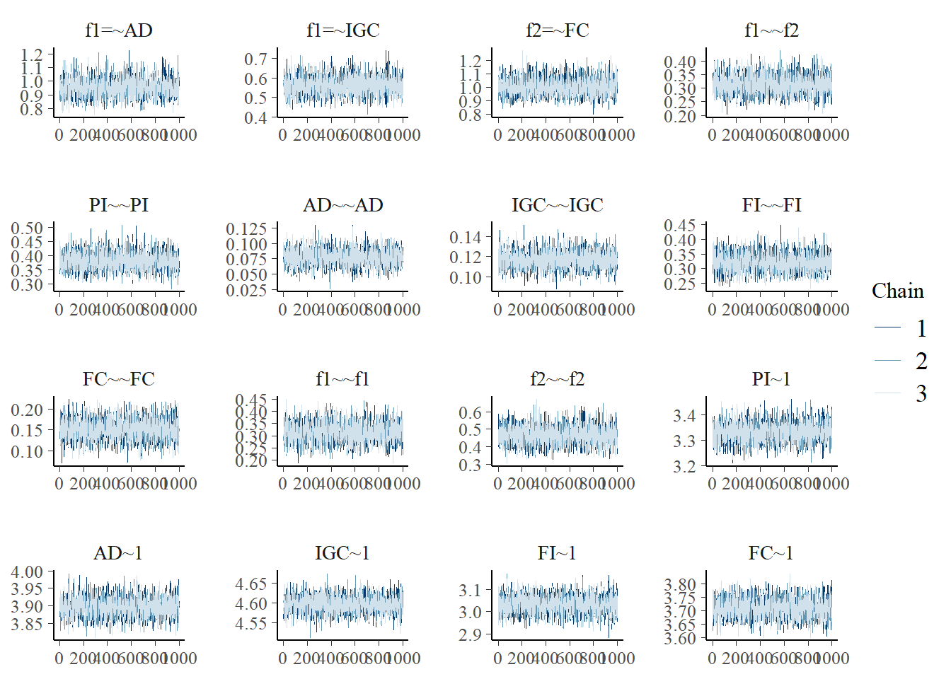
9.9 Indeterminacy in One Factor CFA
# model code
jags.model.cfa.ind <- function(){
######################################################################
# Specify the factor analysis measurement model for the observables
######################################################################
for (i in 1:n){
for(j in 1:J){
mu[i,j] <- tau[j] + ksi[i]*lambda[j] # model implied expectation for each observable
x[i,j] ~ dnorm(mu[i,j], inv.psi[j]) # distribution for each observable
}
}
######################################################################
# Specify the (prior) distribution for the latent variables
######################################################################
for (i in 1:n){
ksi[i] ~ dnorm(kappa, inv.phi) # distribution for the latent variables
}
######################################################################
# Specify the prior distribution for the parameters that govern the latent variables
######################################################################
kappa <- 0 # Mean of factor 1
inv.phi <-1 # Precision of factor 1
phi <- 1/inv.phi # Variance of factor 1
######################################################################
# Specify the prior distribution for the measurement model parameters
######################################################################
for(j in 1:J){
tau[j] ~ dnorm(3, .1) # Intercepts for observables
inv.psi[j] ~ dgamma(5, 10) # Precisions for observables
psi[j] <- 1/inv.psi[j] # Variances for observables
}
for (j in 1:J){
lambda[j] ~ dnorm(1, .1) # prior distribution for the remaining loadings
}
}
# data must be in a list
dat <- read.table("code/CFA-One-Latent-Variable/Data/IIS.dat", header=T)
mydata <- list(
n = 500, J = 5,
x = as.matrix(dat)
)
# initial values
start_values <- list(
list("tau"=c(3.00E+00, 3.00E+00, 3.00E+00, 3.00E+00, 3.00E+00),
"lambda"=c(3.00E+00, 3.00E+00, 3.00E+00, 3.00E+00, 3.00E+00),
"inv.psi"=c(2.00E+00, 2.00E+00, 2.00E+00, 2.00E+00, 2.00E+00)),
list("tau"=c(3.00E+00, 3.00E+00, 3.00E+00, 3.00E+00, 3.00E+00),
"lambda"=c(-3.00E+00, -3.00E+00, -3.00E+00, -3.00E+00, -3.00E+00),
"inv.psi"=c(2.00E+00, 2.00E+00, 2.00E+00, 2.00E+00, 2.00E+00))
)
# vector of all parameters to save
# exclude fixed lambda since it throws an error in
# in the GRB plot
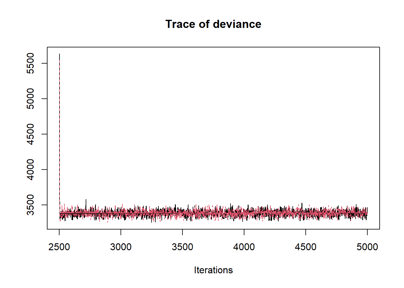
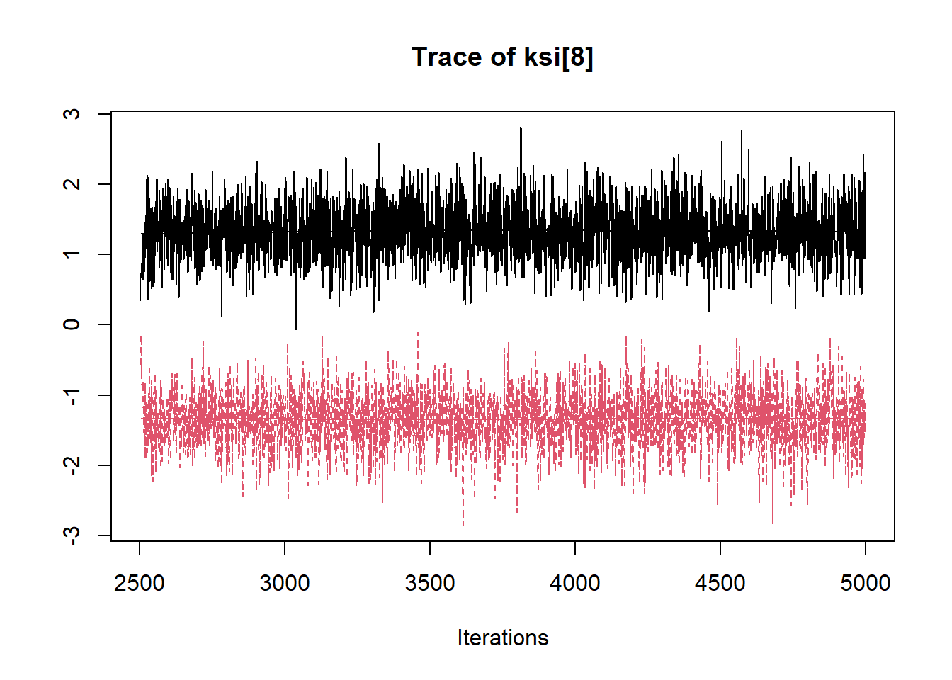
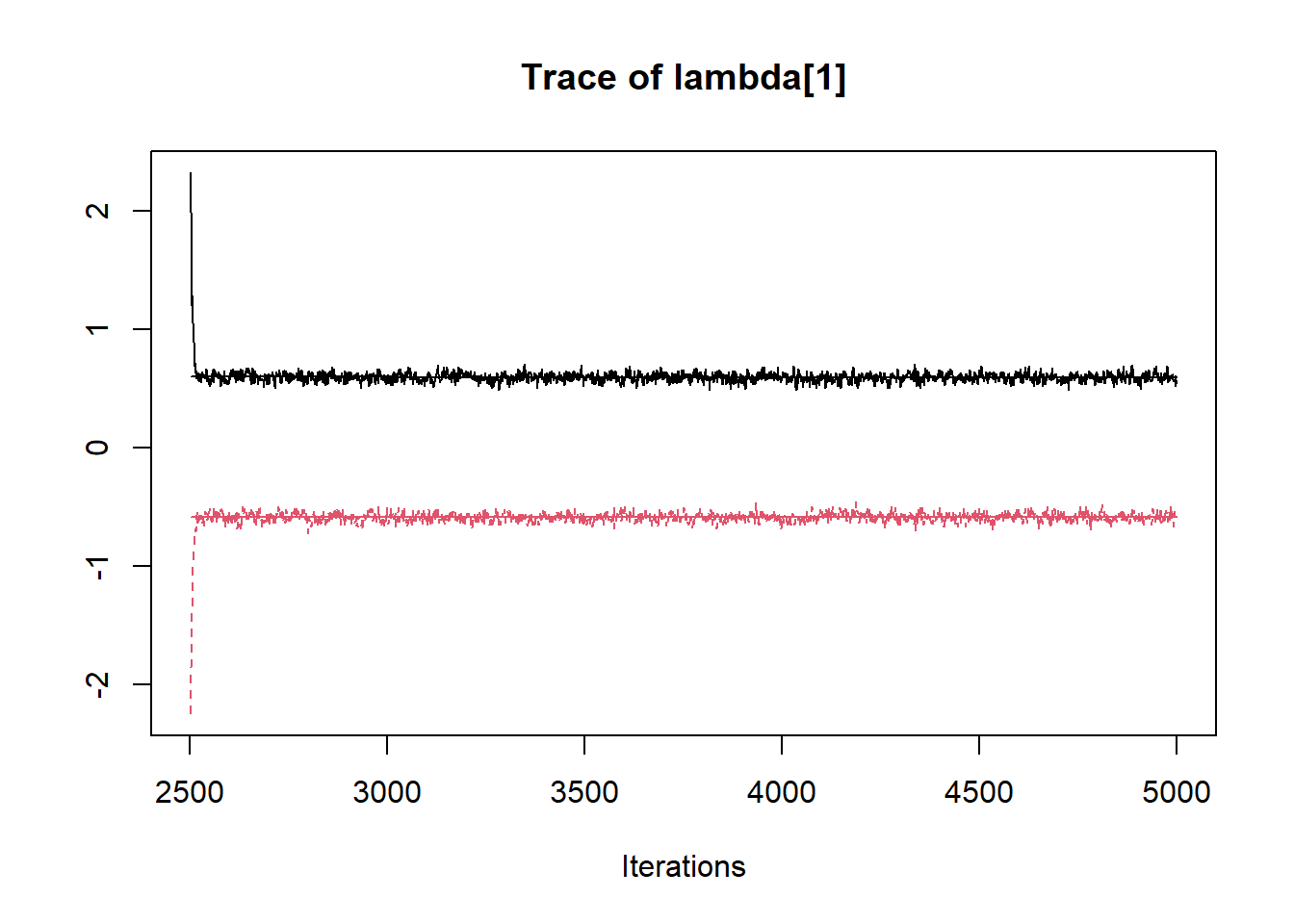
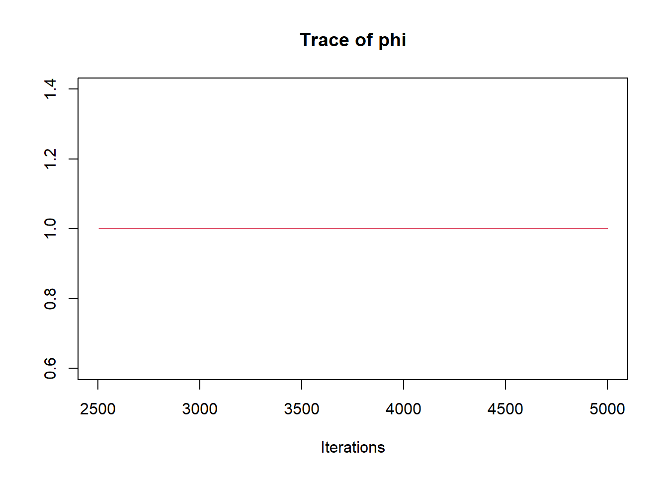
param_save <- c("tau[1]", "lambda[1]", "phi", "psi[1]", "ksi[8]")
# fit model
fit <- jags(
model.file=jags.model.cfa.ind,
data=mydata,
inits=start_values,
parameters.to.save = param_save,
n.iter=5000,
n.burnin = 2500,
n.chains = 2,
n.thin=1,
progress.bar = "none")## Compiling model graph
## Resolving undeclared variables
## Allocating nodes
## Graph information:
## Observed stochastic nodes: 2500
## Unobserved stochastic nodes: 515
## Total graph size: 8029
##
## Initializing model
print(fit)## Inference for Bugs model at "C:/Users/noahp/AppData/Local/Temp/RtmpaGlb2m/model324430075f3.txt", fit using jags,
## 2 chains, each with 5000 iterations (first 2500 discarded)
## n.sims = 5000 iterations saved
## mu.vect sd.vect 2.5% 25% 50% 75% 97.5% Rhat n.eff
## ksi[8] -0.005 1.397 -2.018 -1.336 -0.087 1.332 1.985 8.258 2
## lambda[1] 0.001 0.598 -0.652 -0.591 0.012 0.592 0.651 21.976 2
## phi 1.000 0.000 1.000 1.000 1.000 1.000 1.000 1.000 1
## psi[1] 0.381 0.029 0.327 0.361 0.380 0.400 0.440 1.003 590
## tau[1] 3.332 0.038 3.258 3.307 3.333 3.359 3.405 1.001 2300
## deviance 3383.561 60.868 3300.788 3354.174 3382.183 3410.957 3467.656 1.001 2900
##
## For each parameter, n.eff is a crude measure of effective sample size,
## and Rhat is the potential scale reduction factor (at convergence, Rhat=1).
##
## DIC info (using the rule, pD = var(deviance)/2)
## pD = 1852.3 and DIC = 5235.9
## DIC is an estimate of expected predictive error (lower deviance is better).
# extract posteriors for all chains
jags.mcmc <- as.mcmc(fit)

R2jags::traceplot(jags.mcmc)