4 Normal Distribution Models
This chapter was mainly analytic derivations, but there was one section that did code so I show that in JAGS and Stan.
4.1 Stan Model for mean and variance unknown
The model for mean and variance unknown for normal sampling.
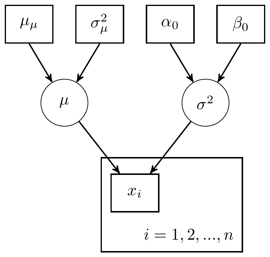
Figure 4.1: DAG with for mean and variance unknown: Variance parameterization
Or, alternatively,
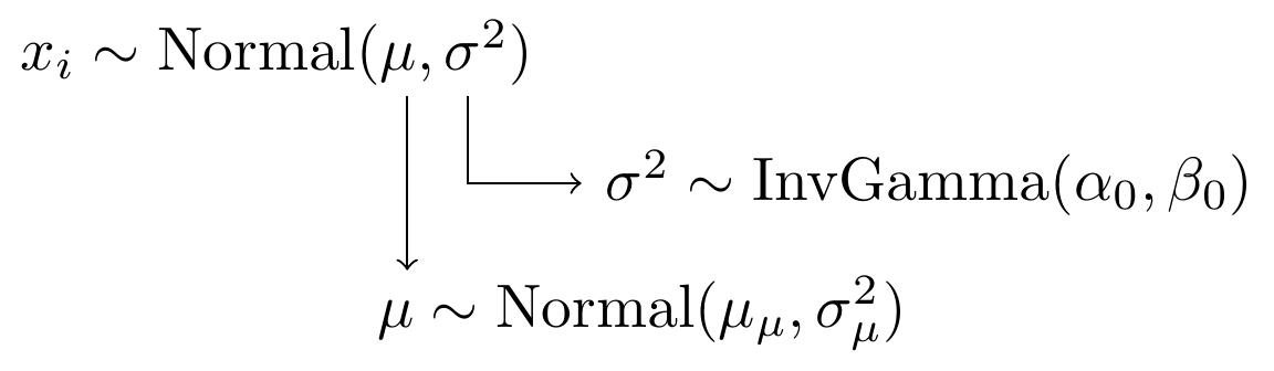
Figure 4.2: Model specification diagram for normal model
model_normal <- '
data {
  int  N;
  real x[N];
  real mu0;
  real sigma0;
  real alpha0;
  real beta0;
}

parameters {
  real mu;
  real<lower=0> sigma;
}

model {
  x ~ normal(mu, sigma);
  mu ~ normal(mu0, sigma0);
  sigma ~ inv_gamma(alpha0, beta0);
}


'
# data must be in a list
mydata <- list(
  N = 10,
  x=c(91, 85, 72, 87, 71, 77, 88, 94, 84, 92),
  mu0 = 75,
  sigma0 = 50,
  alpha0 = 5,
  beta0 = 150
)

# start values
start_values <- function(){
  list(mu=50, sigma=5)
}

# Next, need to fit the model
#   I have explicited outlined some common parameters
fit <- stan(
  model_code = model_normal, # model code to be compiled
  data = mydata,          # my data
  init = start_values,    # starting values
  chains = 4,             # number of Markov chains
  warmup = 1000,          # number of warm up iterations per chain
  iter = 5000,            # total number of iterations per chain
  cores = 2,              # number of cores (could use one per chain)
  refresh = 0             # no progress shown
)

# first get a basic breakdown of the posteriors
print(fit)
## Inference for Stan model: anon_model.
## 4 chains, each with iter=5000; warmup=1000; thin=1;
## post-warmup draws per chain=4000, total post-warmup draws=16000.
##
## mean se_mean sd 2.5% 25% 50% 75% 97.5% n_eff Rhat
## mu 84.04 0.05 4.69 74.66 81.10 84.02 86.97 93.53 8115 1
## sigma 14.79 0.05 3.90 9.19 12.03 14.14 16.80 24.39 7202 1
## lp__ -52.86 0.01 1.05 -55.75 -53.27 -52.54 -52.11 -51.83 5704 1
##
## Samples were drawn using NUTS(diag_e) at Sun Jun 19 17:29:35 2022.
## For each parameter, n_eff is a crude measure of effective sample size,
## and Rhat is the potential scale reduction factor on split chains (at
## convergence, Rhat=1).
# plot the posterior in a
# 95% probability interval
# and 80% to contrast the dispersion
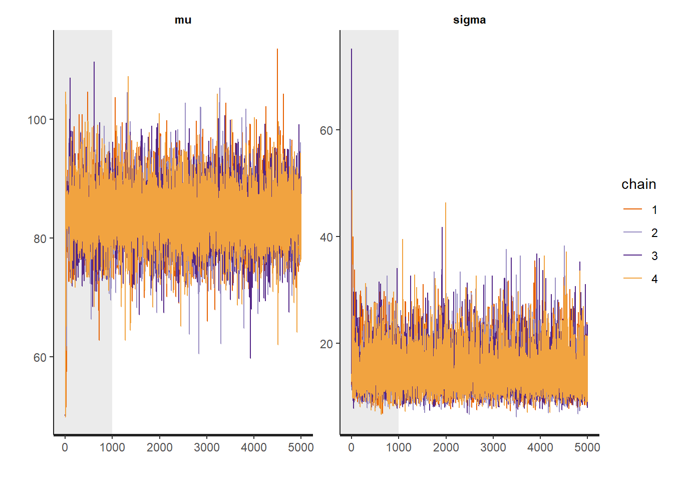
plot(fit)## ci_level: 0.8 (80% intervals)## outer_level: 0.95 (95% intervals)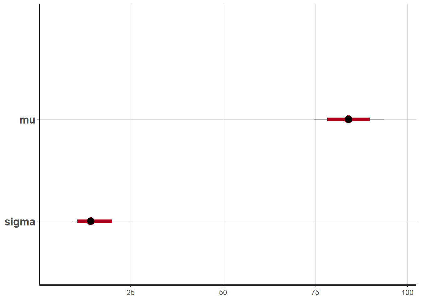
# Gelman-Rubin-Brooks Convergence Criterion
ggs_grb(ggs(fit)) +
   theme_bw() + theme(panel.grid = element_blank())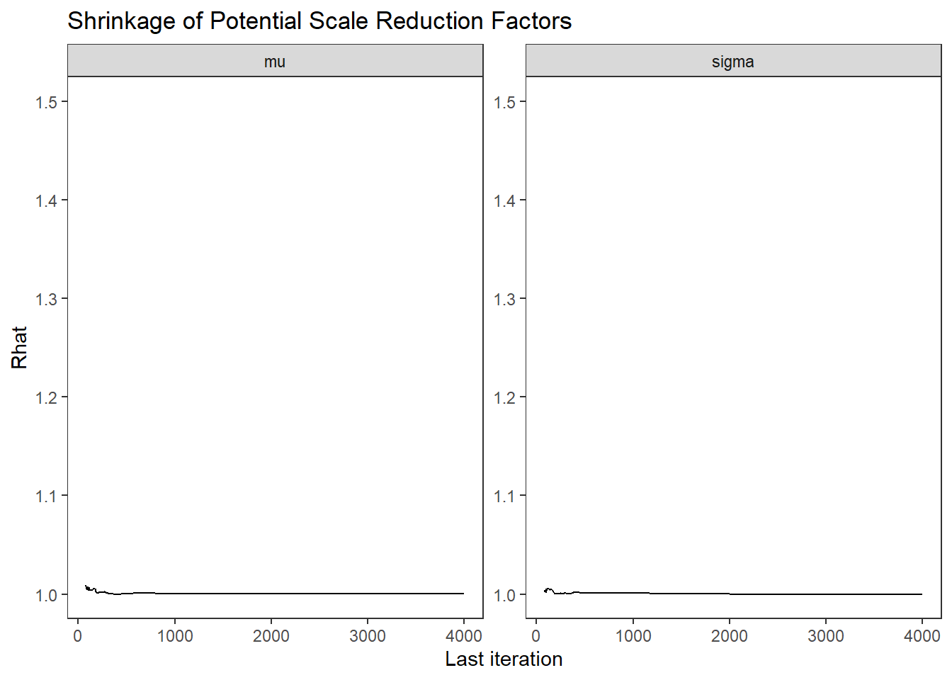
# autocorrelation
ggs_autocorrelation(ggs(fit)) +
   theme_bw() + theme(panel.grid = element_blank())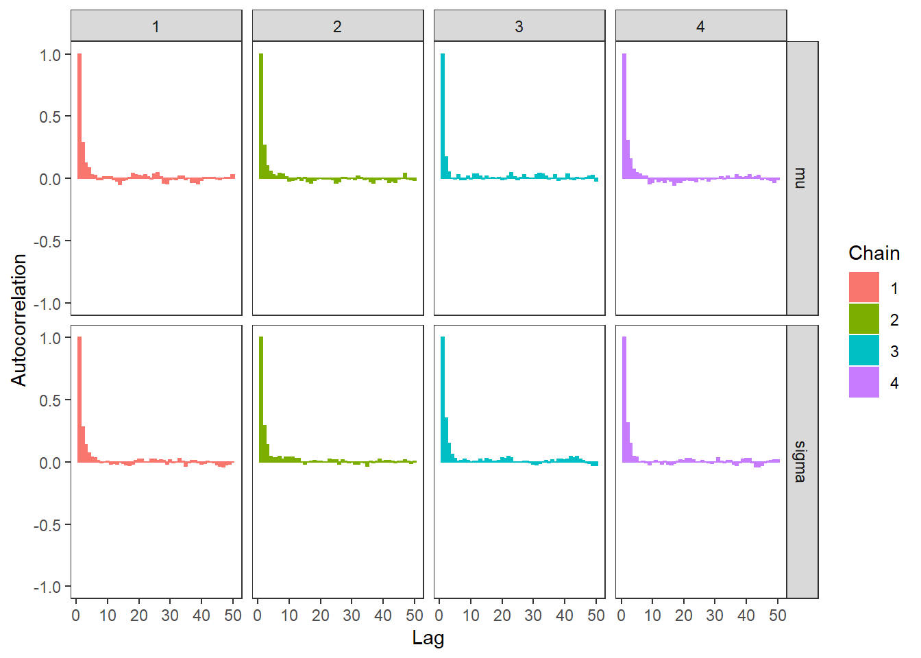
# plot the posterior density
posterior <- as.matrix(fit)

plot_title <- ggtitle("Posterior distributions",
                      "with medians and 80% intervals")
mcmc_areas(
  posterior,
  pars = c("mu", "sigma"),
  prob = 0.8) +
  plot_title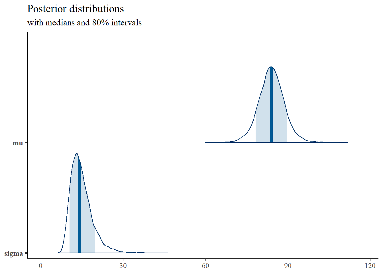
# bivariate plot
posterior <- as.data.frame(posterior)
p <- ggplot(posterior, aes(x=mu, y=sigma))+
  geom_point()+
  theme_bw()+
  theme(panel.grid = element_blank())
p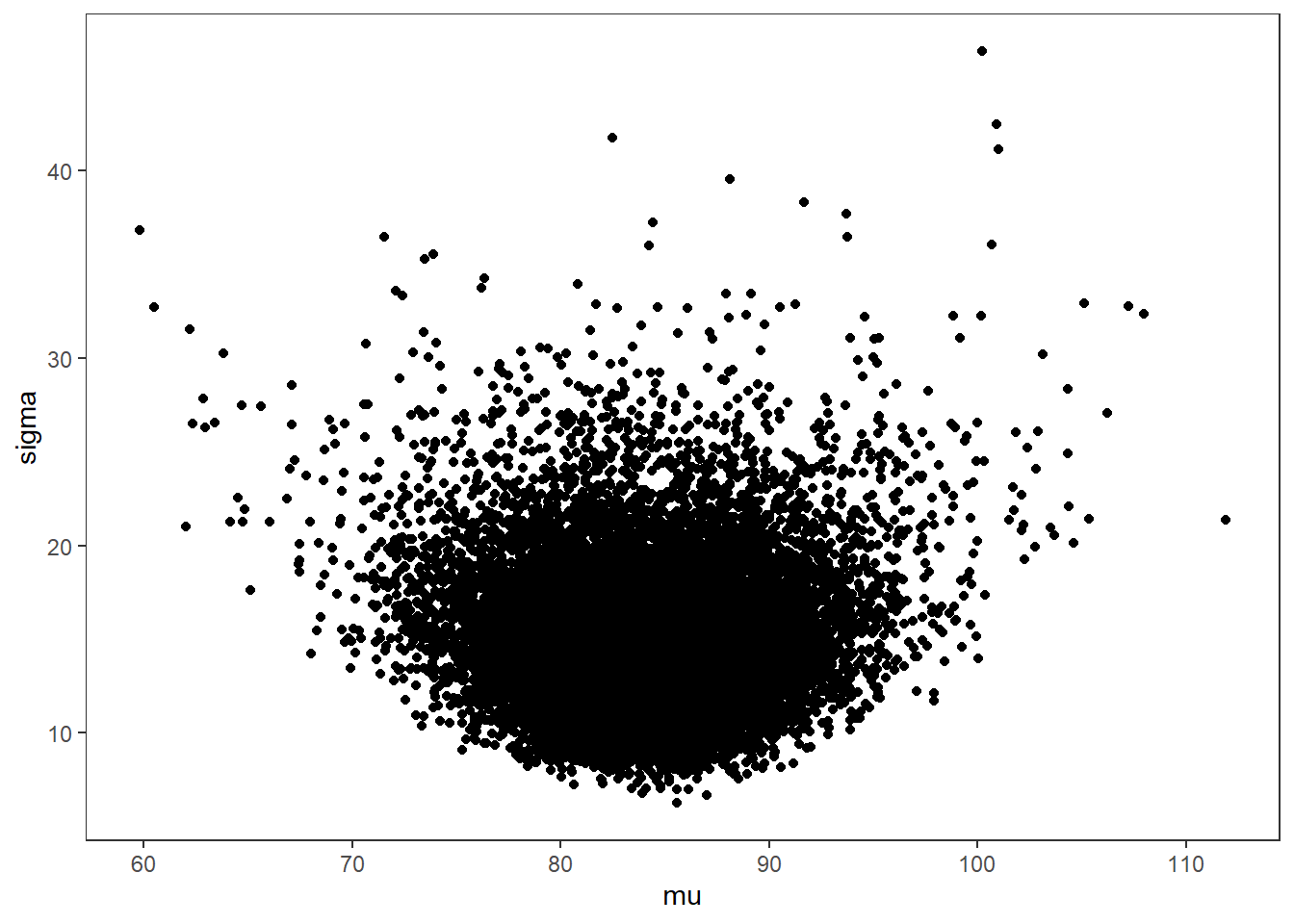
# I prefer a posterior plot that includes prior and MLE
MLE <- c(mean(mydata$x), sd(mydata$x))
prior_mu <- function(x){dnorm(x, 75, 50)}
x.mu <- seq(60.01, 120, 0.01)
prior.mu <- data.frame(mu=x.mu, dens.mu = prior_mu(x.mu))
prior_sig <- function(x){extraDistr::dinvgamma(x, 5, 150)}
x.sig <- seq(0.01, 60, 0.01)
prior.sig <- data.frame(sigma=x.sig, dens.sig = prior_sig(x.sig))
cols <- c("Posterior"="#0072B2", "Prior"="#E69F00", "MLE"= "black")#"#56B4E9", "#E69F00" "#CC79A7"

p1 <- ggplot()+
  geom_density(data=posterior,
               aes(x=mu, color="Posterior"))+
  geom_line(data=prior.mu,
            aes(x=x.mu, y=dens.mu, color="Prior"))+
  geom_vline(aes(xintercept=MLE[1], color="MLE"))+
  scale_color_manual(values=cols, name=NULL)+
  theme_bw()+
  theme(panel.grid = element_blank())

p2 <- ggplot()+
  geom_density(data=posterior,
               aes(x=sigma, color="Posterior"))+
  geom_line(data=prior.sig,
            aes(x=sigma, y=dens.sig, color="Prior"))+
  geom_vline(aes(xintercept=MLE[2], color="MLE"))+
  scale_color_manual(values=cols, name=NULL)+
  theme_bw()+
  theme(panel.grid = element_blank())

p1 + p2 + plot_layout(guides="collect")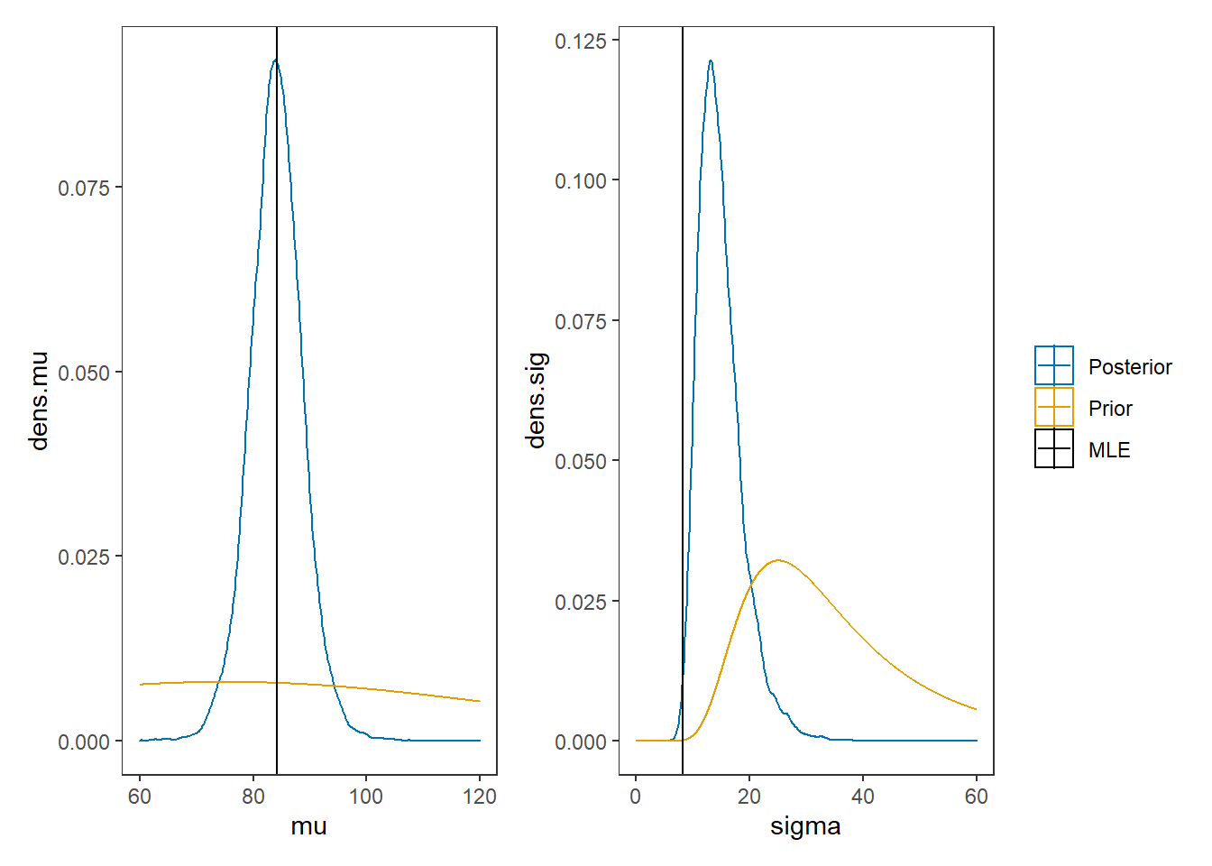
4.2 JAGS Model for mean and variance unknown (precision parameterization)
The model for mean and variance unknown for normal sampling.
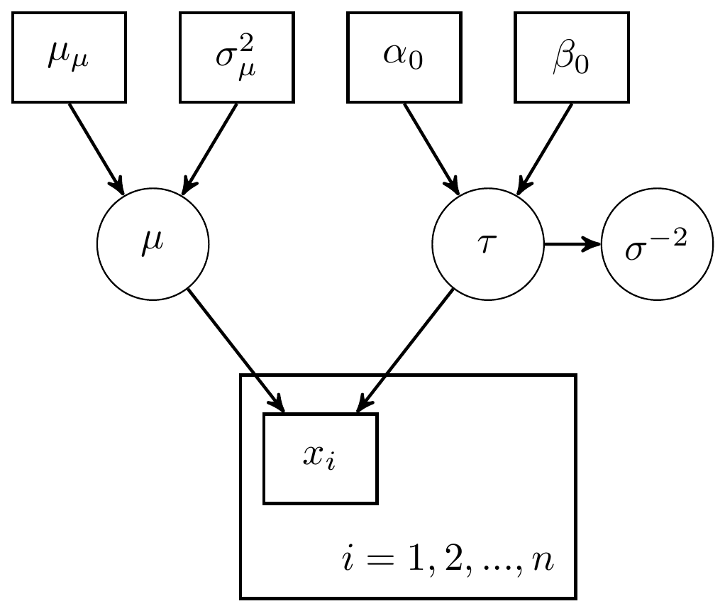
Figure 4.3: DAG with for mean and variance unknown: Precision parameterization
Or, alternatively,
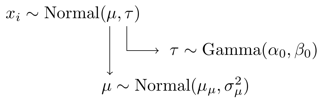
Figure 4.4: Model specification diagram for normal model with precision parameterization
Now for the computation using JAGS
# model code
jags.model <- function(){
  #############################################
  # Conditional distribution for the data
  #############################################

  for(i in 1:n){
    x[i] ~ dnorm(mu, tau)        # conditional distribution of the data
  } # closes loop over subjects


  #############################################
  # Define the prior distributions for the unknown parameters
  # The mean of the data (mu)
  # The variance (sigma.squared) and precision (tau) of the data
  #############################################

  mu ~ dnorm(mu.mu, tau.mu)      # prior distribution for mu

  mu.mu <- 75                          # mean of the prior for mu
  sigma.squared.mu <- 50             # variance of the prior for mu
  tau.mu <- 1/sigma.squared.mu   # precision of the prior for mu


  tau ~ dgamma(alpha, beta)        # precision of the data
  sigma.squared <- 1/tau             # variance of the data
  sigma <- pow(sigma.squared, 0.5) # taking square root

  nu.0 <- 10                           # hyperparameter for prior for tau
  sigma.squared.0 <- 30            # hyperparameter for prior for tau

  alpha <- nu.0/2                    # hyperparameter for prior for tau
  beta <- nu.0*sigma.squared.0/2 # hyperparameter for prior for tau

}
# data
mydata <- list(
  n=10,
  x=c(91, 85, 72, 87, 71, 77, 88, 94, 84, 92))


# starting values
start_values <- function(){
  list("mu"=75, "tau"=0.1)
}

# vector of all parameters to save
param_save <- c("mu", "tau", "sigma")

# fit model
fit <- jags(
  model.file=jags.model,
  data=mydata,
  inits=start_values,
  parameters.to.save = param_save,
  n.iter=4000,
  n.burnin = 1000,
  n.chains = 4,
  n.thin=1,
  progress.bar = "none")
## Compiling model graph
## Resolving undeclared variables
## Allocating nodes
## Graph information:
## Observed stochastic nodes: 10
## Unobserved stochastic nodes: 2
## Total graph size: 26
##
## Initializing model
print(fit)## Inference for Bugs model at "C:/Users/noahp/AppData/Local/Temp/RtmpQR8sbs/model4544158a4038.txt", fit using jags,
## 4 chains, each with 4000 iterations (first 1000 discarded)
## n.sims = 12000 iterations saved
## mu.vect sd.vect 2.5% 25% 50% 75% 97.5% Rhat n.eff
## mu 83.268 2.204 78.845 81.869 83.282 84.725 87.471 1.001 12000
## sigma 7.176 1.238 5.251 6.288 7.007 7.903 10.050 1.001 4000
## tau 0.021 0.007 0.010 0.016 0.020 0.025 0.036 1.001 4000
## deviance 71.212 1.835 69.393 69.897 70.659 71.952 76.128 1.001 12000
##
## For each parameter, n.eff is a crude measure of effective sample size,
## and Rhat is the potential scale reduction factor (at convergence, Rhat=1).
##
## DIC info (using the rule, pD = var(deviance)/2)
## pD = 1.7 and DIC = 72.9
## DIC is an estimate of expected predictive error (lower deviance is better).
# extract posteriors for all chains
jags.mcmc <- as.mcmc(fit)
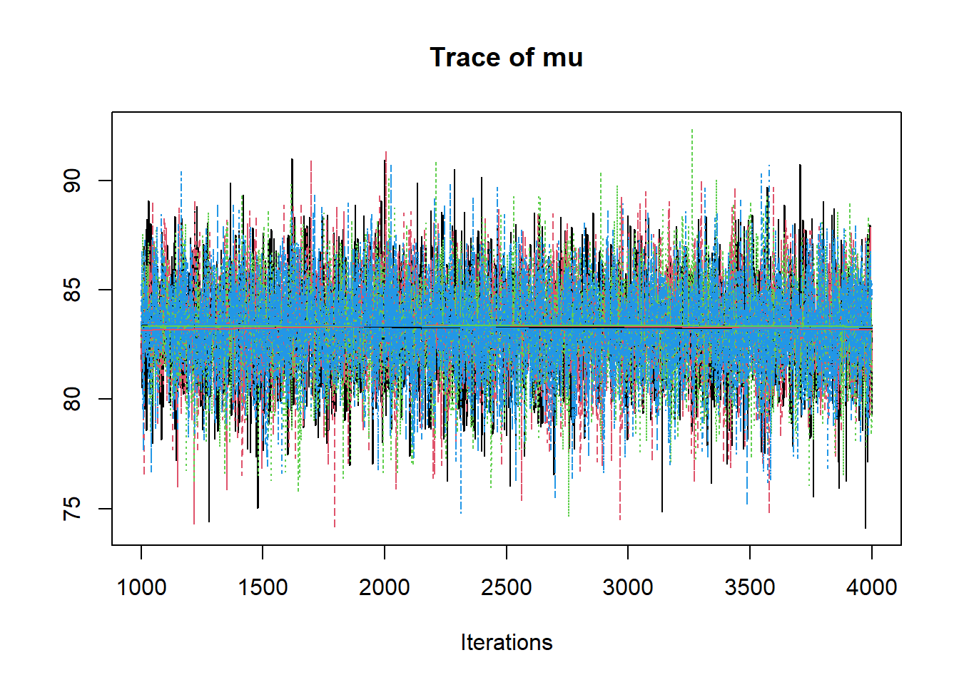
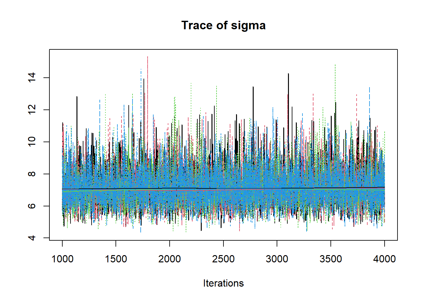
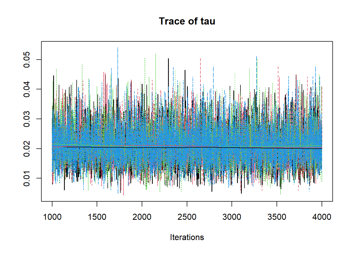
R2jags::traceplot(jags.mcmc)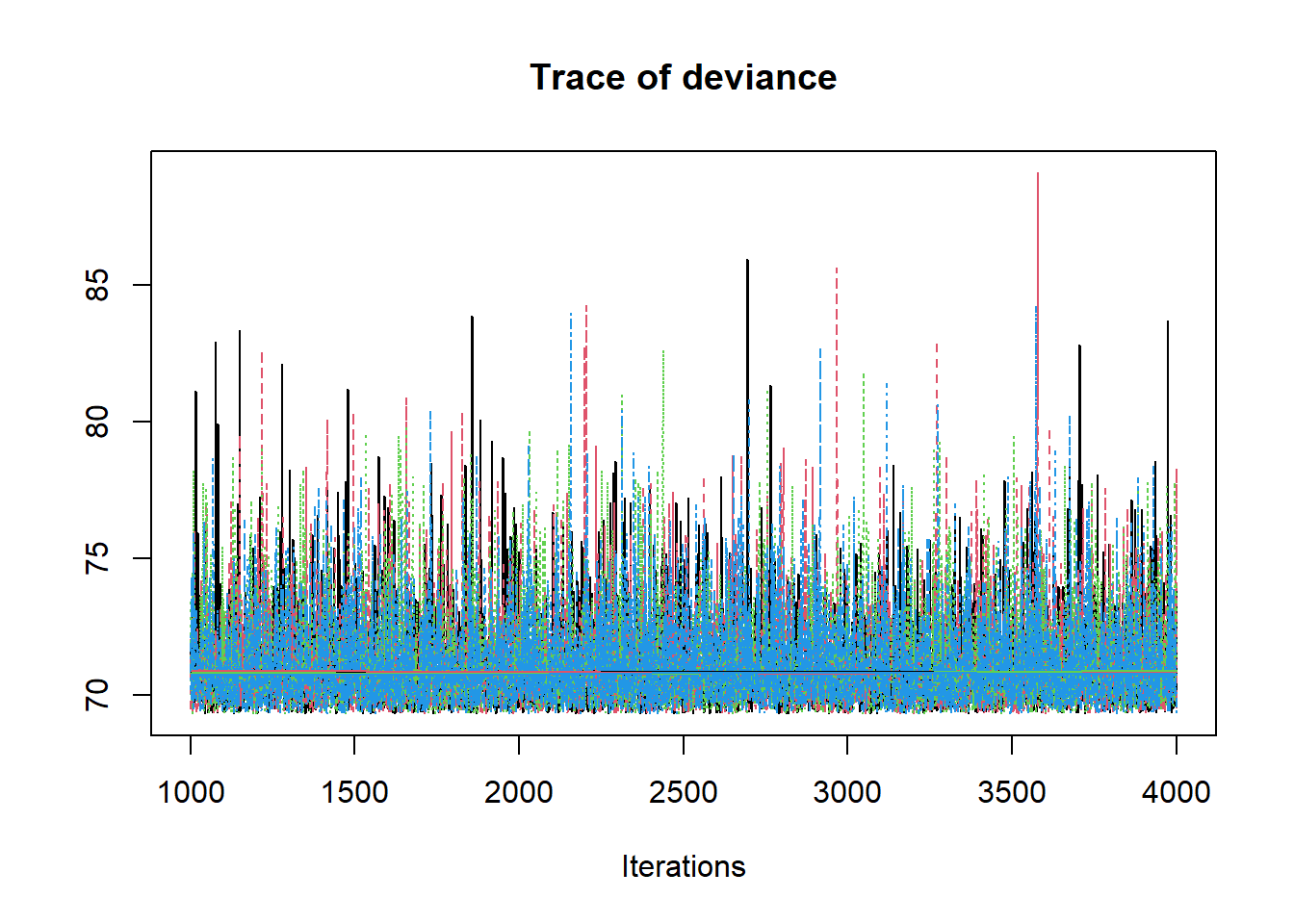
# gelman-rubin-brook
gelman.plot(jags.mcmc)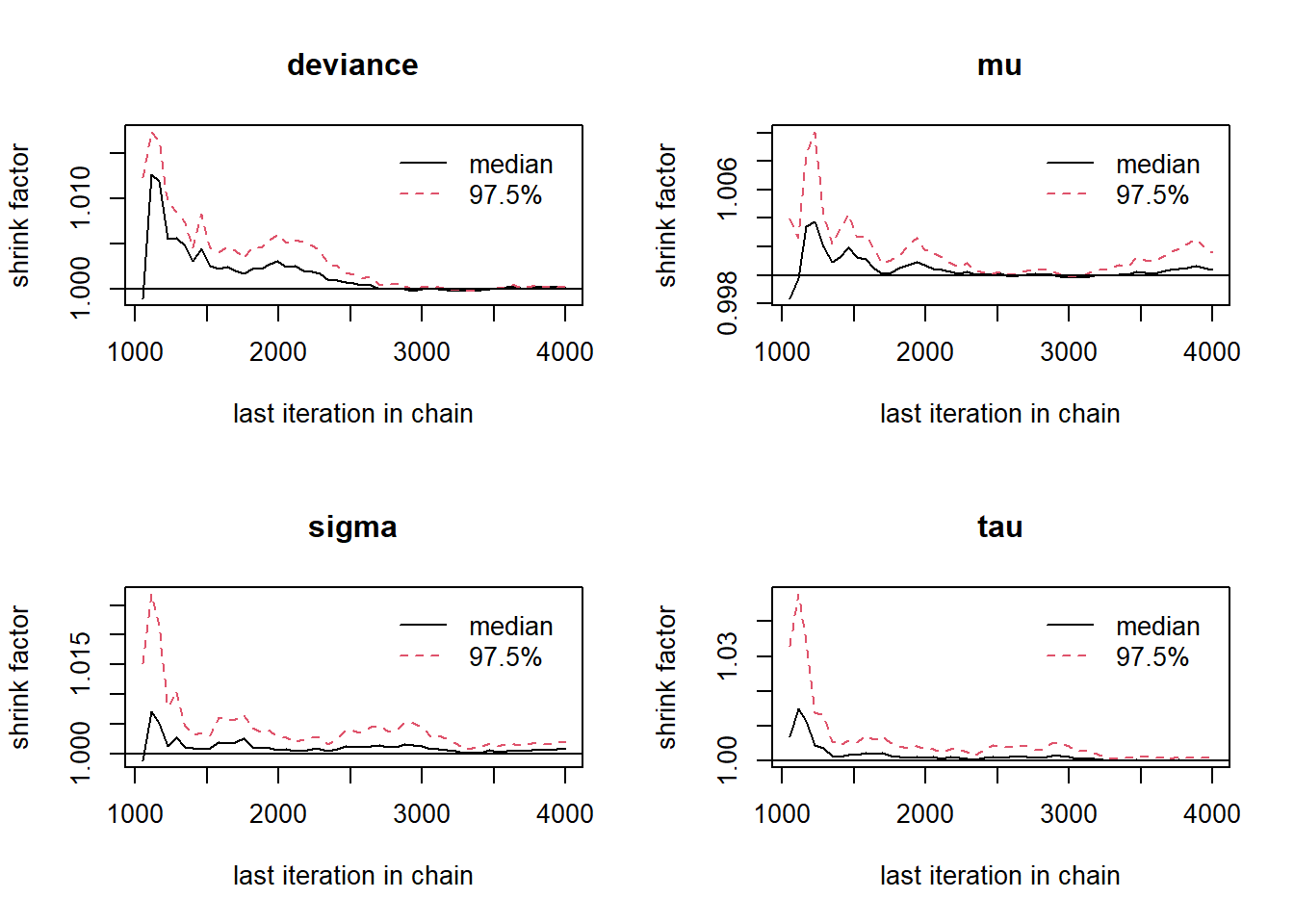
# convert to single data.frame for density plot
a <- colnames(as.data.frame(jags.mcmc[[1]]))
plot.data <- data.frame(as.matrix(jags.mcmc, chains=T, iters = T))
colnames(plot.data) <- c("chain", "iter", a)


plot_title <- ggtitle("Posterior distributions",
                      "with medians and 80% intervals")
mcmc_areas(
  plot.data,
  pars = c("mu"),
  prob = 0.8) +
  plot_title
mcmc_areas(
  plot.data,
  pars = c("tau"),
  prob = 0.8) +
  plot_title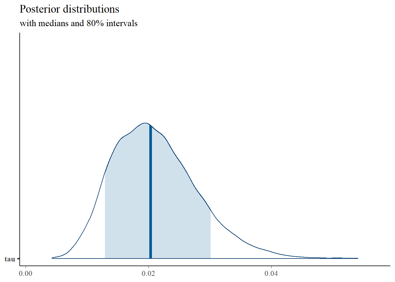
mcmc_areas(
  plot.data,
  pars = c("sigma"),
  prob = 0.8) +
  plot_title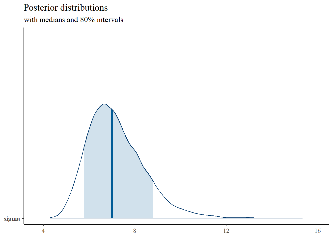
# bivariate plot
p <- ggplot(plot.data, aes(x=mu, y=tau))+
  geom_point()+
  theme_bw()+
  theme(panel.grid = element_blank())
p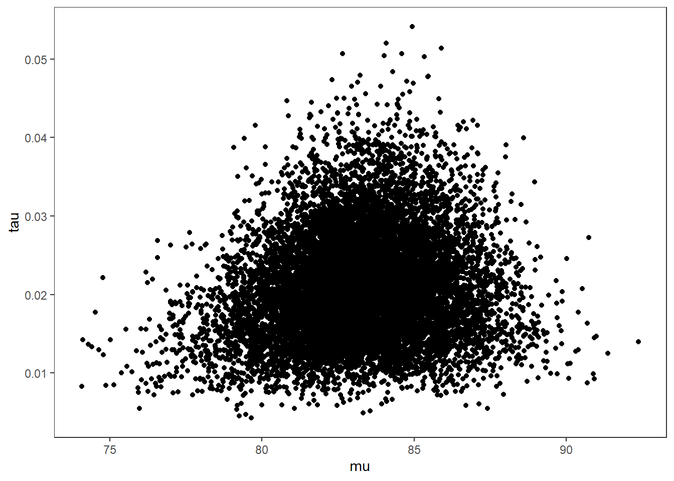
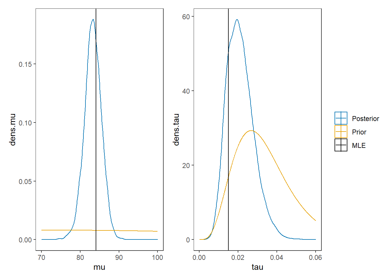
# I prefer a posterior plot that includes prior and MLE
MLE <- c(mean(mydata$x), 1/var(mydata$x))
prior_mu <- function(x){dnorm(x, 75, 50)}
x.mu <- seq(70.01, 100, 0.01)
prior.mu <- data.frame(mu=x.mu, dens.mu = prior_mu(x.mu))
prior_tau <- function(x){dgamma(x, 5, 150)}
x.tau <- seq(0.0001, 0.06, 0.0001)
prior.tau <- data.frame(tau=x.tau, dens.tau = prior_tau(x.tau))
cols <- c("Posterior"="#0072B2", "Prior"="#E69F00", "MLE"= "black")#"#56B4E9", "#E69F00" "#CC79A7"

p1 <- ggplot()+
  geom_density(data=plot.data,
               aes(x=mu, color="Posterior"))+
  geom_line(data=prior.mu,
            aes(x=x.mu, y=dens.mu, color="Prior"))+
  geom_vline(aes(xintercept=MLE[1], color="MLE"))+
  scale_color_manual(values=cols, name=NULL)+
  theme_bw()+
  theme(panel.grid = element_blank())

p2 <- ggplot()+
  geom_density(data=plot.data,
               aes(x=tau, color="Posterior"))+
  geom_line(data=prior.tau,
            aes(x=tau, y=dens.tau, color="Prior"))+
  geom_vline(aes(xintercept=MLE[2], color="MLE"))+
  scale_color_manual(values=cols, name=NULL)+
  theme_bw()+
  theme(panel.grid = element_blank())

p1 + p2 + plot_layout(guides="collect")